Disclaimer
This is not an official Textbook for Data Warehouse.
This is only a reference material with the lecture presented in the class.
If you find any errors, please do email me at chandr34 @ rowan.edu

Fundamentals
- Terms to Know
- Jobs
- Skills needed for DW developer
- Application Tiers
- Operational Database
- What is a Data Warehouse
- Types of Data
- Data Storage Systems
- Data Warehouse 1980 - Current
- Data Warehouse vs Data Mart
- Data Warehouse Architecture
- Data Warehouse Characteristic
- Tools
- Cloud vs On-Premise
- Steps to design a Data Warehouse
Terms to Know
These are some basic terms to know. We will learn lot more going forward.
DBMS - Database Management System
RDBMS - Relational Database Management System
ETL - Extract Transform Load - Back office process for loading data to Data Warehouse.
Bill Inmon - Considered the Father of Data Warehousing.
Ralph Kimball - He’s the father of Dimensional modeling and the Star Schema.
OLTP - Online Transaction Processing. The classic operational database for taking orders, reservations, etc.
OLAP - Online Analytical Processing. Big database providers (IBM, Teradata, Microsoft.. ) started integrating OLAP into their systems.
MetaData - Data about Data.
Data Pipeline - A set of processes that move data from one system to another.
ETL - Extract Transform Load
ELT - Extract Load Transform
Jobs
-
Data Analyst: Plays a crucial role in business decision-making by analyzing data and providing valuable insights, often sourced from a data warehouse.
-
Data Scientist: Employs data warehousing as a powerful tool for modeling, statistical analysis, and predictive analytics, enabling the resolution of complex problems.
-
Data Engineer: Demonstrates precision and dedication in their work by focusing on the design, construction, and maintenance of data pipelines that facilitate the movement of data into and out of a data warehouse.
-
Analyst Engineer: A hybrid role combining the skills of a data analyst and data engineer, often involved in analyzing data and developing the infrastructure to support that analysis.
-
Data Architect: Designs and oversees the implementation of the overall data infrastructure, including data warehouses, to ensure scalability and efficiency.
-
Database Administrator (DBA): This person manages the performance, integrity, and security of databases, including those used in data warehouses.
-
Database Security Analyst: This position focuses on ensuring the security of databases and data warehouses and protecting against threats and vulnerabilities.
-
Database Manager: Oversees the overall management and administration of databases, including those used for data warehousing.
-
Business Intelligence (BI) Analyst: Utilizes data from a data warehouse to generate reports, dashboards, and visualizations that aid business decision-making.
-
AI/ML Engineer: Uses warehouse data to build and deploy machine learning models, particularly in enterprise environments where historical data is crucial.
-
Compliance Analyst: Ensures that data warehousing solutions meet regulatory requirements, especially in industries like finance, healthcare, or insurance.
-
Chief Data Officer (CDO): An executive role responsible for an organization’s data strategy, often overseeing data warehousing as a critical component.
-
Data Doctor: Typically diagnoses and "fixes" data-related issues within an organization. This role might involve data cleansing, ensuring data quality, and resolving inconsistencies or errors in datasets.
-
Data Advocate: Champions the use of data within an organization. They promote data-driven decision-making and ensure that the value of data is recognized and utilized effectively across different departments.
Prefix with Cloud & Big Data
Skills needed
A data warehouse developer is responsible for designing, developing, and maintaining data warehouse systems. To be qualified as a data warehouse developer, a person should possess a combination of technical skills and knowledge in the following areas:
Must-have skills
-
Database Management Systems (DBMS): A strong understanding of relational and analytical database management systems such as Oracle, SQL Server, PostgreSQL, or Teradata.
-
SQL: Proficiency in SQL (Structured Query Language) for creating, querying, and manipulating database objects.
-
Data Modeling: Knowledge of data modeling techniques, including dimensional modeling (star schema, snowflake schema), normalization, and denormalization. Familiarity with tools such as Vertabelo or ERwin, or PowerDesigner is a plus.
-
ETL (Extract, Transform, Load): Experience with ETL processes and tools like Microsoft SQL Server Integration Services (SSIS), Talend, or Informatica PowerCenter for extracting, transforming, and loading data from various sources into the data warehouse.
-
Data Integration: Understanding of data integration concepts and techniques, such as data mapping, data cleansing, and data transformation.
-
Data Quality: Knowledge of data quality management and techniques to ensure data accuracy, consistency, and integrity in the data warehouse.
-
Performance Tuning: Familiarity with performance optimization techniques for data warehouses, such as indexing, partitioning, and materialized views.
-
Reporting and Data Visualization: Experience with reporting and data visualization tools like Tableau, Power BI, or QlikView for creating dashboards, reports, and visualizations to analyze and present data.
-
Big Data Technologies: Familiarity with big data platforms such as Spark and NoSQL databases like MongoDB or Cassandra can be beneficial, as some organizations incorporate these technologies into their data warehousing solutions.
-
Programming Languages: Knowledge of programming languages like Python, Java, or C# can help implement custom data processing logic or integrate with external systems.
-
Cloud Platforms: Experience with cloud-based data warehousing solutions such as Databricks can be a plus as more organizations move their data warehouses to the cloud.
-
Version Control: Familiarity with version control systems like Git or SVN for managing code and collaborating with other developers.
Nice to have skills
In summary, while Linux skills are not a core requirement for a data warehouse developer, they can be valuable for managing, optimizing, and troubleshooting your data warehousing environment.
- Server Management
- Scripting and Automation (AWK, Bash)
- File System and Storage Management
- Networking and Security
- Performance Tuning
- Working with Cloud Platforms
- Deploying and Managing Containers (Docker, Podman, Kubernetes)
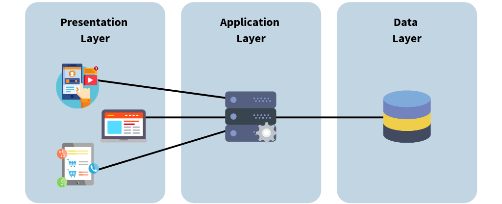
Application Tiers
Where does Database fit in?
- Database Tier: Actual data
- Application Tier: Business logic
- Presentation Tier: Front end (Web, Client, Mobile App)
https://bluzelle.com/blog/things-you-should-know-about-database-caching
Trending Technologies
- Robotics
- AI
- IoT
- Blockchain
- 3D Printing
- Internet / Mobile Apps
- Autonomous Cars - VANET Routing
- VR / AR - Virtual Reality / Augmented Reality
- Wireless Services
- Quantum Computing
- 5G
- Voice Assistant (Siri, Alexa, Google Home)
- Cyber Security
- Big Data Analytics
- Machine Learning
- DevOps
- NoSQL Databases
- Microservices Architecture
- Fintech
- Smart Cities
- E-commerce Platforms
- HealthTech
Do you see any pattern or anything common in these?
Visual Interface & Data
Operational Database
An operational database management system is software that allows users to quickly define, modify, retrieve, and manage data in real time.
While conventional databases rely on batch processing, operational database systems are oriented toward real-time, transactional operations.
Let's take a Retail company that uses several systems for its day-to-day operations.
They buy software from various vendors and manage their business.
- Sales Transactions
- Inventory Management
- Customer Relationship Management
- HR Systems
and so on.
Other Examples:
- Banner Database (Registration)
- eCommerce Database
- Blog Database
- Banking Transactions
What is a Data Warehouse
- Is it a Database?
- Is it Big Data?
- Is it the backend for Visualization?
Yes! Yes! & Yes!

Typical Data Architecture
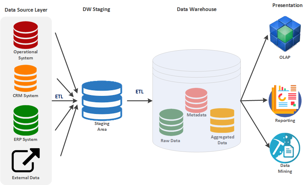
Data Source Layer
Operational System: This includes data from various operational systems like transactional databases. CRM System: Data from customer relationship management systems. ERP System: Data from enterprise resource planning systems. External Data: Data that might come from external sources outside the organization. These sources feed data into the Data Warehouse system. Depending on the source, the data might be structured or unstructured.
DW Staging
Staging Area: This is an intermediate storage area used for data processing during the ETL (Extract, Transform, Load) process. ETL Process: Extract: Data is extracted from various data sources. Transform: The extracted data is transformed into a format suitable for analysis and reporting. This might include cleaning, normalizing, and aggregating the data. Load: The transformed data is then loaded into the Data Warehouse.
Data Warehouse
Raw Data: The unprocessed data loaded directly from the staging area. Metadata: Data about the data, which includes information on data definitions, structures, and rules. Aggregated Data: Summarizing or aggregating data for efficient querying and analysis.
Presentation Layer
**OLAP (Online Analytical Processing): **This tool is used for multidimensional data analysis in the warehouse, enabling users to analyze data from various perspectives. Reporting: Involves generating reports from the data warehouse, often for decision-making and business intelligence purposes. Data Mining: This involves analyzing large datasets to identify patterns, trends, and insights, often used for predictive analytics.
Flow of Data
Data Source Layer → Staging Area: Data is extracted from multiple sources and brought into the staging area. Staging Area → Data Warehouse: The data is transformed and loaded into the data warehouse. Data Warehouse → Presentation Layer: The data is then used for various purposes, such as OLAP, Reporting, and Data Mining.
This architecture ensures that data is collected, processed, and made available for analysis in a structured and efficient manner, facilitating business intelligence and decision-making processes.
Problem Statement
RetailWorld uses different systems for sales transactions, inventory management, customer relationship management (CRM), and human resources (HR). Each system generates a vast amount of data daily.
The company's management wants to make data-driven decisions to improve its operations, optimize its supply chain, and enhance customer satisfaction. However, they face the following challenges:
-
Data Silos: Data is stored in separate systems, making gathering and analyzing information from multiple sources challenging.
-
Inconsistent Data: Different systems use varying data formats, making it hard to consolidate and standardize the data for analysis.
-
Slow Query Performance: As the volume of data grows, querying the operational databases directly becomes slower and impacts the performance of the transactional systems.
-
Limited Historical Data: Operational databases are optimized for current transactions, making storing and analyzing historical data challenging.
Solution
-
Centralized Data Repository: The Data Warehouse consolidates data from multiple sources, breaking down data silos and enabling a unified view of the company's information.
-
Consistent Data Format: Data is cleaned, transformed, and standardized to ensure consistency and accuracy across the organization.
-
Improved Query Performance: The Data Warehouse is optimized for analytical processing, allowing faster query performance without impacting the operational systems.
-
Historical Data Storage: The Data Warehouse can store and manage large volumes of historical data, enabling trend analysis and long-term decision-making.
-
Enhanced Reporting and Analysis: The Data Warehouse simplifies the process of generating reports and conducting in-depth analyses, providing insights into sales trends, customer preferences, inventory levels, and employee performance.
Key Features
- They are used for storing historical data.
- Low Latency / Response time is fast.
- Data consistency and quality of data.
- Used with Business Intelligence, Data Analysis & Data Science.
By doing all the above, it answers some of the questions the business/needs.
- Sales of particular items this month compared to last month?
- Top 3 best-selling products of the quarter?
- How is the internet traffic before the pandemic / during the pandemic?
It's read-only for end-users and upper management.
Who are the end users?
- Data Analysts
- Data Scientists.
Data Size
A query can range from a few thousand rows to billion rows.
Need for Data Warehouse
Amazon CEO wants to know the sales of the new Kindle Scribe reader they launched this year compared to other eReaders in the next 30 mins.
Where do we look for this info?
- Transactional databases use every resource to serve customers. Querying on them may slow down a customer's request.
- Also, they are Live databases. So they may or may not have historical data.
- Chances are data format may differ for each region/country in which Amazon is doing business in.
It's not just Amazon; it's everywhere.
- Airlines
- Bank Transactions / ATM transactions
- Restaurant chains, and so on.
Companies will have multiple databases that are not linked with each other for specific reasons.
- Sales Database
- Customer Service Database
- Marketing Database
- Inventory Database
- Human Resources Database
There is no reason for linking HR data to Sales data, but the CFO might need this info for budgeting.
Fun Qn: How many times have you received Marketing mail/email from the same company you have an account with?
Current State of the Art
The business world decided as follows.
-
A Database should exist just for doing BI & Strategic reports.
-
It should be separated from the operational / transaction database for the day-to-day running of the business.
-
It should encompass all aspects of the business (sales, inventory, hr, customer service…)
-
An enterprise-wide standard definition for every field name in every table.
- Example: employee number should be identical across DB. empNo, eNo,EmployeeNum.. empID not acceptable.
-
Metadata database (data about data) defining assumptions about each field, describing transformations performed and cleansing operations, etc.
- Example: If US telephone, it should be nnn-nnn-nnnn or (nnn) nnn-nnnn
-
Data Warehouse is read-only to its end users so that everyone will use the same data, and there will be no mismatch between teams.
-
Fast access, even if it's big data.
How its done?
-
Operational databases for tracking sales, inventory, support calls, chat, and email. (Relational / NoSQL)
-
The Back Office team (ETL team) gathers data from multiple sources, cleans it, transforms it, massages the missing, and stores it in the Staging database.
- If the phone number is not in the format, then format it.
- If the email address is not linked to the chat/phone record, read it from the Customer and update it.
-
Staging database: Working database where all the work is done to the data. It then dumps to the data warehouse, which is visible as “read-only” to end users.
-
Data Analysts then build reports using Data Warehouse.
Back to the original question.
If all of these things are done right, Amazon's CEO can get the report in less than 30 minutes without interfering with business operations. 👍
Types of Data
- Structured Data (rows/columns CSV, Excel)
- Semi-Structured Data (JSON / XML)
- Unstructured Data (Video, Audio, Document, Email)
Structured Data
| ID | Name | Join Date |
|---|---|---|
| 101 | Rachel Green | 2020-05-01 |
| 201 | Joey Tribianni | 1998-07-05 |
| 301 | Monica Geller | 1999-12-14 |
| 401 | Cosmo Kramer | 2001-06-05 |
Semi-Structured Data
JSON
[
   {
      "id":1,
      "name":"Rachel Green",
      "gender":"F",
      "series":"Friends"
   },
   {
      "id":"2",
      "name":"Sheldon Cooper",
      "gender":"M",
      "series":"BBT"
   }
]
XML
<?xml version="1.0" encoding="UTF-8"?>
<actors>
   <actor>
      <id>1</id>
      <name>Rachel Green</name>
      <gender>F</gender>
      <series>Friends</series>
   </actor>

   <actor>
      <id>2</id>
      <name>Sheldon Cooper</name>
      <gender>M</gender>
      <series>BBT</series>
   </actor>
</actors>
Unstructured Data
- Text Logs: Server logs, application logs.
- Social Media Posts: Tweets, Facebook comments.
- Emails: Customer support interactions.
- Audio/Video: Customer call recordings and marketing videos.
- Customer Reviews: Free-form text reviews.
- Images: Product images user profile pictures.
- Documents: PDFs, Word files.
- Sensor Data: IoT data streams.
These can be ingested into modern data warehouses for analytics, often after some preprocessing. For instance, text can be analyzed with NLP before storing, or images can be processed into feature vectors.
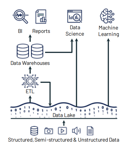
Data Storage Systems
Data Lake
A place where you dump all forms of data of your business.
Structured / Un Structured / Semi-Structured.
Example
- Customer service chat logs, voice recordings, email, website comments, social media.
- Need a cheap way to store different types of data in large quantities.
- Data is not needed now, but planning to use it for later use.
- Larger organizations need all kinds of data to analyze and improve business.
Data Warehouse
- Data Warehouse - Stores already modeled/structured data and ready for use.
- Data from the Warehouse can be used for analyzing its operational data.
- There will be developers to support the data.
- It’s multi-purpose storage for different use cases.
Data Mart
A subset of Data Warehouse for a specific use case.
A specific group of users uses it, so it is more secure and performs better.
Example: Pandemic Analysis
Dependent Data Marts - constructed from an existing data warehouse.
Example: Grocery / School Supplies
Independent Data Marts - built from scratch and operated in silos.
Example: Mask / Glove Sales
Hybrid Data Marts - Mix and match both.
Data Warehouse 1980 - Current
Data Warehouses (1980 - 2000):
Pros
- High Quality Data.
- Standard modeling technique (star schema/Kimball).
- Reliability through ACID transactions.
- Very good fit for business intelligence.
Cons
- Closed Formats.
- Support only SQL.
- No support for Machine Learning.
- No streaming support.
- Limited scaling support.
Data Lakes (2010 - 2020)
Pros
- Support for open formats.
- Can support all data types & their use cases.
- Scalability through underlying cloud storage.
- Support for Machine Learning & AI.
Cons
- Weak schema support.
- No ACID transaction support.
- Low data quality.
- Leads to "Data Swamps".
Lakehouses (2020 and beyond):
Pros
- Support for both BI and ML/AI workloads.
- Standard Storage Format.
- Reliability through ACID transactions.
- Scalability through underlying cloud storage.
Cons
- Cost Considerations.
- Data Governance and Security.
- Performance Overhead. (Due to ACID transactions)
Data Warehouse vs Data Mart
| Data Warehouse | Data Mart |
|---|---|
| Independent application / system | Specific to support one system. |
| Contains detailed data. | Mostly aggregated data. |
| Involves top-down/bottom-up approach. | Involves bottom-up approach. |
| Adjustable and exists for an extended period of time. | Restricted for a project / shorter duration of time. |
Data Warehouse Architecture
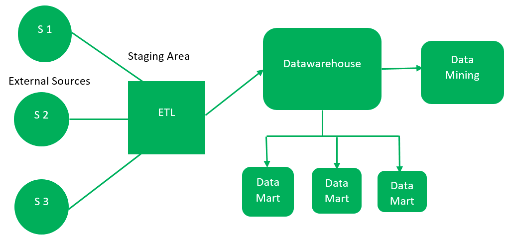
Top-Down Approach
This method begins with developing a comprehensive enterprise data warehouse (EDW) consolidating all organizational data. This central warehouse creates data marts to serve specific business units or functions. The top-down approach ensures a unified, consistent data model across the enterprise but typically requires more upfront investment in time and resources.
External Sources (ETL) >> Data Warehouse >> Data Mining
                                         >> Data Mart 1
                                         >> Data Mart 2
In the words of Inmon
"Data Warehouse as a central repository for the complete organization and data marts are created from it after the complete data warehouse has been created."
src: https://www.geeksforgeeks.org/data-warehouse-architecture/
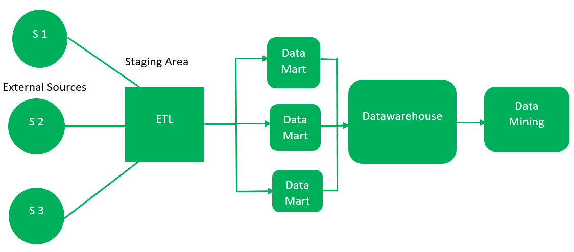
Bottom-Up Approach
This approach starts by creating small, specific data marts for individual business units. These data marts are designed to meet the immediate analytical needs of departments. Over time, these marts are integrated into a comprehensive enterprise data warehouse (EDW). The bottom-up approach is agile and allows quick wins but can lead to challenges integrating data marts into a cohesive system.
External Sources (ETL)     >> Data Mart 1  >> Data Warehouse >> Data Mining
                           >> Data Mart 2
Kimball gives this approach: data marts are created first and provide a thin view for analysis, and a data warehouse is created after complete data marts have been created.
src: https://www.geeksforgeeks.org/data-warehouse-architecture/
Summary
Each approach has its advantages and trade-offs, with the bottom-up being more iterative and flexible, while the top-down offers a more structured and holistic view of the organization’s data.
Examples:
Top Down - Popular big retail stores likely to follow this architecture. As they have build a centralized data warehouse that feeds their stores. Similarly Financial organlizations like Banks may take top-down approach.
Bottom Up - Popular OTT have such models. Initially bring movies, then add their own production and add third party providers.
Data Warehouse Characteristic
Characteristics
- Subject Oriented
- Integrated
- Time-Variant
- Non-Volatile
- Data Loading (ETL)
- Data Access (Reporting / BI)
Functions
- Data Consolidation
- Data Cleaning
- Data Integration
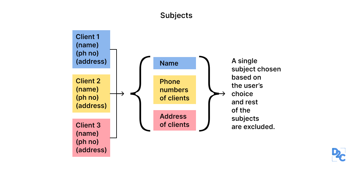
Subject Oriented
src: https://unstop.com/blog/characteristics-of-data-warehouse
Data analysis for a business's decision-makers can be done quickly by constricting to a particular subject area of the Data warehouse.
Do not add unwanted info on subjects for decision-making.
When analyzing customer information, it's crucial to focus on the relevant data and avoid unnecessary details, such as food habbits, which can distract from the main task.
Integrated
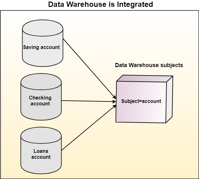
Multiple Source Systems:
In most organizations, data is stored across various systems. For example, a bank might have separate systems for savings accounts, checking accounts, and loans. Each system is designed to serve a specific purpose and might have its own database, schema, and data formats.
Unified Subject Areas:
The data warehouse is a centralized repository where data from these different source systems is brought together. This integration is not just about storing the data in one place; it involves transforming and aligning the data to be analyzed.
Consistency and Standardization:
During integration, the data is often standardized to ensure consistency. For example, account numbers might be formatted differently in the source systems, but they are unified in a standard format in the data warehouse. This standardization is crucial for accurate reporting and analysis.
Benefits:
Holistic View: The data warehouse provides a comprehensive view of a subject by integrating data from different sources. For example, a bank can now analyze a customer's relationship across all accounts rather than looking at each in isolation.
Improved Decision-Making: With integrated data, organizations can perform more sophisticated analyses, leading to better decision-making. For example, they can understand a customer's total exposure by analyzing their savings, checking, and loan accounts together.
Efficiency: Analysts and business users can access all the relevant data in one place without needing to query multiple systems.
Time Variant

Data warehouses, unlike operational databases, are designed with a unique ability to maintain a comprehensive historical record of data. This feature not only allows for trend analysis and historical reporting but also ensures the reliability of the system for comparison over time.
For example, if a customer changes their address, a data warehouse will keep old and new addresses, along with timestamps indicating when the change occurred.
Data warehouses often include a time dimension, allowing users to analyze data across different periods. This could include daily, monthly, quarterly, or yearly trends, providing insights into how data changes over time.
Non Volatile
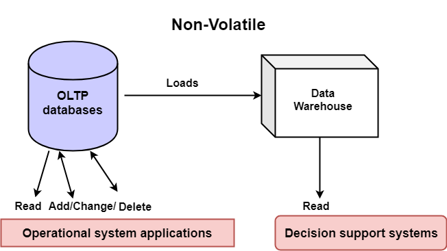
Non-Volatile Nature: The data warehouse does not allow modifications to the data once it is loaded. This characteristic ensures that historical data is preserved for long-term analysis.
The cylinder on the left side of the diagram represents OLTP databases, which are typically used in operational systems. These databases handle day-to-day transactions, such as reading, adding, changing, or deleting data. OLTP systems are optimized for fast transaction processing.
The cube represents the data warehouse, a dedicated repository designed for analysis and reporting. Unlike OLTP systems, the data warehouse is non-volatile, meaning that once data is loaded into the warehouse, it remains stable and is not updated or deleted. This stability is a key feature, ensuring that historical data is preserved intact for analysis over time.
Tools
Traditional Solutions
- SQL Server
- Oracle
- PostgreSQL
- IBM DB2
- Teradata
- Informatica
- SAP HANA
Cloud Solutions
- Databricks
- Snowflake
- Microsoft Fabric
- Google BigQuery
- Amazon Redshift
ETL/ELT Tools
- Talend
- Apache NiFi
- Fivetran
- Apache Airflow (orchestrator)
Data Integration and Data Prep
- Alteryx
- Trifacta
- dbt (data build tool)
BI and Analytics Tools
- Tableau
- QlikView
- Power BI
- Looker
Data Lakes
- AWS Lake Formation
- Azure Data Lake
- Google Cloud Storage
- Apache Hadoop (HDFS)
Data Cataloging and Governance
- Unity Catalog
- Apache Atlas
- Collibra
- Alation
- Informatica Data Catalog
Big Data Technologies
- Apache Spark
- Apache Hive
- Apache Impala
- Apache HBase
- Presto
Cloud vs On-Premise
| Feature | Cloud Datawarehouse | On-Premise |
|---|---|---|
| Scalability | Instant Up / Down, Scale In / Out | Reconfiguring / purchasing hardware, software, etc. |
| Availability | Up to 99.99% | Depends on infrastructure. |
| Security | Provided by cloud provider | Depends on the competence of the in-house IT team. |
| Performance | Serve multiple geo locations, helps query performance | Scalability challenge |
| Cost-effectiveness | No hardware / initial cost. Pay only for usage. | Requires significant initial investment, salary. |
src: https://www.scnsoft.com/analytics/data-warehouse/cloud
Steps to design a Data Warehouse
- Gather Requirements
- Environment (Physical / Cloud)
- Dev
- Test
- Prod
- Data Modeling
- Star Schema
- Snowflake Schema
- Galaxy Schema
- Choose ETL - ELT Solution
- OLAP Cubes or Not
- Visualization Tool
- Query Performance
Gather Requirements
-
DW is subject-oriented.
-
Needs data from all related sources. DW is valuable as the data contained within it.
-
Talk to groups and align goals with the overall project.
-
Could you determine the scope of the project and how it helps the business?
-
Discover future needs with the data and technology solution.
-
Disaster Recovery model.
-
Security (threat detection, mitigation, monitoring)
-
Anticipate compliance needs and mitigate regulatory risks.
Environment
-
Need separate environments for Development, Testing, and Production.
-
Development & Testing will have some % of sample data from Production.
-
Testing and Production will have a similar HW environment. (Cloud / In house)
-
Nice to have a similar environment for development.
-
Track changes, indexes, and query changes are done in the lower environment.
-
DR environment is part of the Production release.
-
Suppose it's in-house; deploy it in different data centers. If it's cloud, deploy it in different regions.
Data Modeling
-
Data Modeling is a process to visualize the data warehouse.
-
It helps to set standards in naming conventions, creating relationships between datasets, and establishing compliance and security.
-
Most Complex phase in data warehouse design.
-
Recollect Top - Down vs. Bottom - Up that decision plays a vital role.
-
Data Modelling typically starts at the data mart level and then branches out to the data warehouse.
-
Three popular data models for data warehouses
- Star Schema
- Galaxy Schema
- Snowflake Schema
ETL / ELT Solution
ETL
- Extract
- Transform
- Load
ETL plays a vital part in moving data across. Many ways ETL can be implemented.
Popular ones
GUI Tools such as
- SSIS
- Pentaho
- Talend
- Scripting Tools such as Bash, Python.
ELT
- Extract
- Load
- Transform
In big data platforms such as Hadoop, and Spark, you can load a JSON, or CSV file and start using them as is. This technology can even parse compressed .gz / .bz2 files
Extensively used when dealing with Semi-Structured databases.
Register with Databricks community edition
Online Analytic Processing
In OLAP cube data can be pre-calculated and pre-aggregated, making analysis faster.
Usually, data is organized in row and column format.
OLAP contains multi-dimensional data, with data from different data sources.

There are 4 types of analytical operations in OLAP
Roll-up: Consolidation, aggregation. Data from different cities can be rolled up to the state/country level.
Drill-down: Opposite of roll-up. If you have data by year, you can analyze monthly, weekly, and daily trends.
Slice-dice: Take one dimension of the data from the cube and create a sub-cube.
If data from various products / various quarters are available take one quarter alone and work with it.
Pivot: Rotating the data axes. Basically swapping the x and y-axis of the data.
Front End
Visualization - the primary reason for creating data warehouses.
Popular Premium BI tools.
- Tableau
- PowerBI
- Looker
Check Data Warehouse Tools for more details.
Query Optimization
These are some basic best practices. There is lot more to discuss in future sessions.
-
Retrieve only necessary rows.
-
Do not use *; instead, specify the columns.
-
Create views so users will control the data pull as well as security.
-
Filter first and Join later.
-
Filter first and Group later.
-
Monitor queries regularly for performance.
-
Index only when needed. Please don't index unwanted columns.
RDBMS
- Data Model
- Online vs Batch
- DSL vs GPL
- Storage Formats
- File Formats
- DuckDB
- DuckDB Sample - 01
- DuckDB Sample - 02
- DuckDB - Date Dimension
- Practice using SQLBolt
Data Model
Data Models: Is used to define how the logical structure of a database is modeled.
Entity: A Database entity is a thing, person, place, unit, object, or any item about which the data should be captured and stored in properties, workflow, and tables.
Attributes: Properties of Entity.
Example:
Entity: Student
Attributes: id, name, join date
Student
| student id | name | join date |
|---|---|---|
| 101 | Rachel Green | 2000-05-01 |
| 201 | Joey Tribianni | 1998-07-05 |
| 301 | Monica Geller | 1999-12-14 |
| 401 | Cosmo Kramer | 2001-06-05 |
Entity Relationship Model
Student
| student id | name | join date |
|---|---|---|
| 101 | Rachel Green | 2000-05-01 |
| 201 | Joey Tribianni | 1998-07-05 |
| 301 | Monica Geller | 1999-12-14 |
| 401 | Cosmo Kramer | 2001-06-05 |
Courses
| student id | semester | course |
|---|---|---|
| 101 | Semester 1 | DBMS |
| 101 | Semester 1 | Calculus |
| 201 | Semester 1 | Algebra |
| 201 | Semester 1 | Web |
One to One Mapping
erDiagram
    Student {
        int student_id PK
        string name
        date join_date
    }

    Studentdetails {
        int student_id PK
        string SSN
        date DOB
    }

    Student ||--|| Studentdetails : "1 to 1"
Student
| student id | name | join date |
|---|---|---|
| 101 | Rachel Green | 2000-05-01 |
| 201 | Joey Tribianni | 1998-07-05 |
| 301 | Monica Geller | 1999-12-14 |
| 401 | Cosmo Kramer | 2001-06-05 |
Studentdetails
| student id | SSN | DOB |
|---|---|---|
| 101 | 123-56-7890 | 1980-05-01 |
| 201 | 236-56-4586 | 1979-07-05 |
| 301 | 365-45-9875 | 1980-12-14 |
| 401 | 148-89-4758 | 1978-06-05 |
For every row on the left-hand side, there will be only one matching entry on the right-hand side.
For student id 101, you will find one SSN and one DOB.
One to Many Mapping
erDiagram
    Student {
        int student_id PK
        string name
        date join_date
    }

    Address {
        int address_id PK
        int student_id FK
        string address
        string address_type
    }

    Student ||--o{ Address : "has"
Student
| student id | name | join date |
|---|---|---|
| 101 | Rachel Green | 2000-05-01 |
| 201 | Joey Tribianni | 1998-07-05 |
| 301 | Monica Geller | 1999-12-14 |
| 401 | Cosmo Kramer | 2001-06-05 |
Address
| student id | address id | address | address type |
|---|---|---|---|
| 101 | 1 | 1 main st, NY | Home |
| 101 | 2 | 4 john blvd,NJ | Dorm |
| 301 | 3 | 3 main st, NY | Home |
| 301 | 4 | 5 john blvd,NJ | Dorm |
| 201 | 5 | 12 center st, NY | Home |
| 401 | 6 | 11 pint st, NY | Home |
What do you notice here?
Every row on the left-hand side has one or more rows on the right-hand side.
For student id 101, you will notice the home address and Dorm address.
Many to Many Mapping
erDiagram
    Student {
        int student_id PK
        string name
        date join_date
    }

    Course {
        string course_id PK
        string course_name
    }

    StudentCourses {
        int student_id FK
        string course_id FK
    }

    Student ||--o{ StudentCourses : enrolls
    Course ||--o{ StudentCourses : offered_in
Student
| student id | name | join date |
|---|---|---|
| 101 | Rachel Green | 2000-05-01 |
| 201 | Joey Tribianni | 1998-07-05 |
| 301 | Monica Geller | 1999-12-14 |
| 401 | Cosmo Kramer | 2001-06-05 |
Student Courses
| student id | course id |
|---|---|
| 101 | c1 |
| 101 | c2 |
| 301 | c1 |
| 301 | c3 |
| 201 | c3 |
| 401 | c4 |
Courses
| course id | course name |
|---|---|
| c1 | DataBase |
| c2 | Web Programming |
| c3 | Big Data |
| c4 | Data Warehouse |
What do you notice here?
Students can take more than one course, and courses can have more than one student.
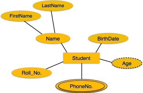
Attributes
Types of Attributes
Simple Attribute - Atomic Values.
An attribute that cannot be divided further.
Example: ssn
Composite Attribute
Made up of more than one simple attribute.
Example: firstname + mi + lastname
Derived Attribute
Calculated from existing attributes.
Age: Derived from DOB
Multivalued Attribute
An attribute that can have multiple values for a single entity (e.g., PhoneNumbers for a person).
src: https://www.tutorialspoint.com/dbms/er_diagram_representation.htm
Student: Entity
Name: Composite Attribute
Student ID: Simple Attribute
Age: Derived Attribute
PhoneNo: MultiValued Attribute
(The Student can have more than one phone number)
Keys
Primary Key
The Attribute helps to identify a row in an entity uniquely.
It cannot be empty and cannot have duplicates.
| student id | name | join date |
|---|---|---|
| 101 | Rachel Green | 2020-05-01 |
| 201 | Joey Tribianni | 1998-07-05 |
| 301 | Monica Geller | 1999-12-14 |
| 401 | Cosmo Kramer | 2001-06-05 |
Based on the above data, which attribute can be PK?
any column (as its just four rows)
If we extend the dataset to 10000 rows, which can be PK?
yes student id
Composite Key
A Primary key that consists of two or more attributes is known as a **** composite key.
| student id | course id | name |
|---|---|---|
| 101 | C1 | Rachel Green |
| 101 | C2 | Rachel Green |
| 201 | C2 | Monica Geller |
| 201 | C3 | Cosmo Kramer |
Do you know how to find the unique row?
The combination of StudentID + CourseID makes it unique.
Unique Key
Unique keys are similar to Primary Key, except it can allow one NULL.
Transaction
What is a Transaction?
A transaction can be defined as a group of tasks.
A simple task is the minimum processing unit that cannot be divided further.
Example: Transfer $500 from X account to Y account.
Open_Account(X)
Old_Balance = X.balance
New_Balance = Old_Balance - 500
X.balance = New_Balance
Close_Account(X)

Open_Account(Y)
Old_Balance = B.balance
New_Balance = Old_Balance + 500
Y.balance = New_Balance
Close_Account(Y)
States of Transaction
src: https://www.tutorialspoint.com/dbms/dbms_transaction.htm
src: www.guru99.com
- Active: When the transaction's instructions are running, the transaction is active.
- Partially Committed: After completing all the read and write operations, the changes are made in the main memory or local buffer.
- Committed: It is the state in which the changes are made permanent on the DataBase.
- Failed: When any instruction of the transaction fails.
- Aborted: The changes are only made to the local buffer or main memory; hence, these changes are deleted.
ACID
ACID Complaint
Atomicity: All or none. Changes all or none.
Consistency: Never leaves the database in a half-finished state. Deleting a customer is not possible before deleting related invoices.
Isolation: Separates a transaction from another. Transactions are isolated; they occur independently without interference. One change will not be visible to another transaction.
Durability: Recover from an abnormal termination. Once the transaction is completed, data is written to disk and persists when the system fails. DB returns to a consistent state when restarted due to abnormal termination.
Example
Atomicity
Example: Transferring money between two bank accounts. If you transfer $100 from Account A to Account B, the transaction must ensure that either the debit from Account A and credit to Account B occur or neither occurs. If any error happens during the transaction (e.g., system crash), the transaction will be rolled back, ensuring that no partial transaction is completed.
Consistency
Example: Enforcing database constraints, such as ensuring that a field that stores a percentage can only hold values between 0 and 100. If an operation tries to insert a value of 110, it will fail because it violates the consistency rule of the database schema.
Isolation:
Example: Two transactions that concurrently update the same set of rows in a database. Transaction A updates a row; before it commits, Transaction B also tries to update the same row. Depending on the isolation level (e.g., Serializable), Transaction B may be required to wait until Transaction A commits or rolls back to avoid data inconsistencies, ensuring that transactions do not interfere with each other.
Durability:
Example: After a transaction is committed, such as a user adding an item to a shopping cart in an e-commerce application, the data must be permanently saved to the database. Even if the server crashes immediately after the commit, the added item must remain in the shopping cart once the system is back online.
Online/Realtime vs Batch
Online Processing
An online system handles transactions when they occur and provides output directly to users. It is interactive.
Use Cases
E-commerce Websites:
Use Case: Processing customer orders. Example: When a customer places an order, the system immediately updates inventory, processes the payment, and provides an order confirmation in real time. Any delay could lead to issues like overselling stock or customer dissatisfaction.
Online Banking:
Use Case: Fund transfers and account balance updates. Example: When a user transfers money between accounts, the transaction is processed immediately, and the balance is updated in real-time. Real-time processing is crucial to ensure the funds are available immediately and that the account balance reflects the latest transactions.
Social Media Platforms:
Use Case: Posting updates and notifications. Example: When a user posts a new status or comment, it should be instantly visible to their followers. Notifications about likes, comments, or messages are also delivered in real time to maintain user engagement.
Ride-Sharing Services (e.g., Uber, Lyft):
Use Case: Matching drivers with passengers. Example: When a user requests a ride, the system matches them with a nearby driver in real time, providing immediate feedback on the driver's location and estimated arrival time.
Fraud Detection Systems:
Use Case: Monitoring transactions for fraudulent activities. Example: Credit card transactions are monitored in real time to detect unusual patterns and prevent fraud before they are completed.
Batch Processing
Data is processed in groups or batches. Batch processing is typically used for large amounts of data that must be processed on a routine schedule, such as paychecks or credit card transactions.
A batch processing system has several main characteristics: collect, group, and process transactions periodically.
Batch programs require no user involvement and require significantly fewer network resources than online systems.
Use Cases
End-of-Day Financial Processing:
Use Case: Reconciling daily transactions. Example: Banks often batch process all the day's transactions at the end of the business day to reconcile accounts, generate statements, and update records. This processing doesn't need to be real-time but must be accurate and comprehensive.
Data Warehousing and ETL Processes:
Use Case: Extracting, transforming, and loading data into a data warehouse. Example: A retail company may extract sales data from various stores, transform it to match the warehouse schema, and load it into a centralized data warehouse. This process is typically done in batches overnight to prepare the data for reporting and analysis the next day.
Payroll Processing:
Use Case: Calculating employee salaries. Example: Payroll systems typically calculate and process salaries in batches, often once per pay period. Employee data (hours worked, overtime, deductions) is collected over the period and processed in a single batch job.
Inventory Updates:
Use Case: Updating inventory levels across multiple locations. Example: A chain of retail stores might batch-process inventory updates at the end of each day. Each store's sales data is sent to a central system, where inventory levels are adjusted in batches to reflect the day's sales.
Billing Systems:
Use Case: Generating customer bills. Example: Utility companies often generate customer bills at the end of each month. Usage data is collected throughout the month, and bills are generated in batch processing jobs, which are then sent to customers.
DSL vs GPL
GPL - General Programming Language.  Python / JAVA / C++

One tool can be used to do many things.

DSL - Domain-Specific Language. HTML / SQL / JQ / AWK /...

Specific tools to do a specific job.

src: https://tomassetti.me/domain-specific-languages/"
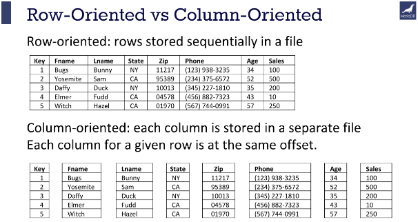
Storage Formats
| Account number | Last name | First name | Purchase (in dollars) |
|---|---|---|---|
| 1001 | Green | Rachel | 20.12 |
| 1002 | Geller | Ross | 12.25 |
| 1003 | Bing | Chandler | 45.25 |
Row Oriented Storage
In a row-oriented DBMS, the data would be stored as
1001,Green,Rachel,20.12;1002,Geller,Ross,12.25;1003,Bing,Chandler,45.25
Best suited for OLTP - Transaction data.
Columnar Oriented Storage
1001,1002,1003;Green,Geller,Bing;Rachel,Ross,Chandler;20.12,12.25,45.25
Best suited for OLAP - Analytical data.
-
Compression: Since the data in a column tends to be of the same type (e.g., all integers, all strings), and often similar values, it can be compressed much more effectively than row-based data.
-
Query Performance: Queries that only access a subset of columns can read just the data they need, reducing disk I/O and significantly speeding up query execution.
-
Analytic Processing: Columnar storage is well-suited for analytical queries and data warehousing, which often involve complex calculations over large amounts of data. Since these queries often only affect a subset of the columns in a table, columnar storage can lead to significant performance improvements.
src: https://mariadb.com/resources/blog/why-is-columnstore-important/
File Formats
CSV/TSV
Pros
- Tabular Row storage.
- Human-readable is easy to edit manually.
- Simple schema.
- Easy to implement and parse the file(s).
Cons
- No standard way to present binary data.
- No complex data types.
- Large in size.
JSON
Pros
- Supports hierarchical structure.
- Most languages support them.
- Widely used in Web
Cons
- More memory usage due to repeatable column names.
- Not very splittable.
- Lacks indexing.
Parquet
Parquet is a columnar storage file format optimized for use with Apache Hadoop and related big data processing frameworks. Twitter and Cloudera developed it to provide a compact and efficient way of storing large, flat datasets.
Best for WORM (Write Once Read Many).
The key features of Parquet are:
- Columnar Storage: Parquet is optimized for columnar storage, unlike row-based files like CSV or TSV. This allows it to efficiently compress and encode data, which makes it a good fit for storing data frames.
- Schema Evolution: Parquet supports complex nested data structures, and the schema can be modified over time. This provides much flexibility when dealing with data that may evolve.
- Compression and Encoding: Parquet allows for highly efficient compression and encoding schemes. This is because columnar storage makes better compression and encoding schemes possible, which can lead to significant storage savings.
- Language Agnostic: Parquet is built from the ground up for use in many languages. Official libraries are available for reading and writing Parquet files in many languages, including Java, C++, Python, and more.
- Integration: Parquet is designed to integrate well with various big data frameworks. It has deep support in Apache Hadoop, Apache Spark, and Apache Hive and works well with other data processing frameworks.
In short, Parquet is a powerful tool in the big data ecosystem due to its efficiency, flexibility, and compatibility with a wide range of tools and languages.
Difference between CSV and Parquet
| Aspect | CSV (Comma-Separated Values) | Parquet |
|---|---|---|
| Data Format | Text-based, plain text | Columnar, binary format |
| Compression | Usually uncompressed (or lightly compressed) | Highly compressed |
| Schema | None, schema-less | Strong schema enforcement |
| Read/Write Efficiency | Row-based, less efficient for column operations | Column-based, efficient for analytics |
| File Size | Generally larger | Typically smaller due to compression |
| Storage | More storage space required | Less storage space required |
| Data Access | Good for sequential access | Efficient for accessing specific columns |
| Example Size (1 GB) | Could be around 1 GB or more depending on compression | Could be 200-300 MB (due to compression) |
| Use Cases | Simple data exchange, compatibility | Big data analytics, data warehousing |
| Support for Data Types | Limited to text, numbers | Rich data types (int, float, string, etc.) |
| Processing Speed | Slower for large datasets, particularly for queries on specific columns | Faster, especially for column-based queries |
| Tool Compatibility | Supported by most tools, databases, and programming languages | Supported by big data tools like Apache Spark, Hadoop, etc. |
Parquet Compression
- Snappy (default)
- Gzip
Snappy
- Low CPU Util
- Low Compression Rate
- Splittable
- Use Case: Hot Layer
- Compute Intensive
GZip
- High CPU Util
- High Compression Rate
- Splittable
- Use Case: Cold Layer
- Storage Intensive
DuckDB
DuckDB is an in-process SQL database management system designed for efficient analytical query processing.
Its a single file DB, no need of Client / Server setup.
Its like SQLLite on Steroids.
Install Duck DB
https://duckdb.org/#quickinstall
Key Features
In-Process Execution: DuckDB operates entirely within your application process, eliminating the need for a client-server setup. This makes it highly efficient for embedded analytics.
Columnar Storage: DuckDB uses a columnar storage format, unlike traditional row-based databases. This allows it to handle analytical queries more efficiently, as operations can simultaneously be performed on entire columns.
SQL Compatibility: DuckDB's wide range of SQL features makes it a breeze to use for anyone familiar with SQL. It can handle complex queries, joins, and aggregations without requiring specialized query syntax, ensuring a comfortable and familiar experience.
Integration and Ease of Use: DuckDB is designed to integrate easily into various environments. It supports multiple programming languages, including Python, R, and C++, and can be used directly within data science workflows.
Scalability: DuckDB, while optimized for in-process execution, is more than capable of scaling to handle large datasets. This reassures you that it's a reliable choice for lightweight analytics and exploratory data analysis (EDA).
Extensibility: The database supports user-defined functions (UDFs) and extensions, allowing you to extend its capabilities to fit your needs.
Limitations
- Limited Transaction Support
- Concurrency Limitations
- No Client-Server Model
- Lack of Advanced RDBMS Features
- Not Designed for Massive Data Warehousing
Duckdb Sample - 01
Launch Duckdb
duckdb
.open newdbname.duckdb
CREATE TABLE employees (
    id INTEGER PRIMARY KEY,
    name VARCHAR NOT NULL,
    email VARCHAR UNIQUE,
    department VARCHAR,
    salary DECIMAL(10, 2) CHECK (salary > 0)
);

INSERT INTO employees (id,name, email, department, salary) VALUES
(1,'Rachel Green', 'rachel.green@friends.com', 'Fashion', 55000.00);

INSERT INTO employees (id,name, email, department, salary) VALUES
(2,'Monica Geller', 'monica.geller@friends.com', 'Culinary', 62000.50);

INSERT INTO employees (id,name, email, department, salary) VALUES
(3,'Phoebe Buffay', 'phoebe.buffay@friends.com', 'Massage Therapy', 48000.00);

INSERT INTO employees (id,name, email, department, salary) VALUES
(4,'Joey Tribbiani', 'joey.tribbiani@friends.com', 'Acting', 40000.75);

INSERT INTO employees (id,name, email, department, salary) VALUES
(5,'Chandler Bing', 'chandler.bing@friends.com', 'Data Analysis', 70000.25);

INSERT INTO employees (id,name, email, department, salary) VALUES
(6,'Ross Geller', 'ross.geller@friends.com', 'Paleontology', 65000.00);
select * from employees
- .databases or show databases;
- .tables or show tables;
- .mode list
- .mode table
- .mode csv
- summarize employees;
- summarize select name,email from employees;
- .exit
CREATE SEQUENCE dept_id_seq;

drop table if exists departments;

CREATE TABLE departments (
    id INTEGER PRIMARY KEY DEFAULT nextval('dept_id_seq'),
    dept_name VARCHAR NOT NULL
);

insert into departments(dept_name) values('Fashion');
insert into departments(dept_name) values('Culinary');
insert into departments(dept_name) values('Massage');
insert into departments(dept_name) values('Acting');
insert into departments(dept_name) values('Data Analysis');
insert into departments(dept_name) values('Paleontology');


CREATE SEQUENCE emp_id_seq;

DROP TABLE if exists employees;

CREATE TABLE if not exists  employees (
    id INTEGER PRIMARY KEY DEFAULT nextval('emp_id_seq'),
    name VARCHAR NOT NULL,
    email VARCHAR UNIQUE,
    department VARCHAR,
    salary DECIMAL(10, 2) CHECK (salary > 0),
    hire_date DATE DEFAULT CURRENT_DATE,
);


INSERT INTO employees (name, email, department, salary) VALUES
('Rachel Green', 'rachel.green@friends.com', 'Fashion', 55000.00);

INSERT INTO employees (name, email, department, salary) VALUES
('Monica Geller', 'monica.geller@friends.com', 'Culinary', 62000.50);

INSERT INTO employees (name, email, department, salary) VALUES
('Phoebe Buffay', 'phoebe.buffay@friends.com', 'Massage Therapy', 48000.00);

INSERT INTO employees (name, email, department, salary) VALUES
('Joey Tribbiani', 'joey.tribbiani@friends.com', 'Acting', 40000.75);

INSERT INTO employees (name, email, department, salary) VALUES
('Chandler Bing', 'chandler.bing@friends.com', 'Data Analysis', 70000.25);

INSERT INTO employees (name, email, department, salary) VALUES
('Ross Geller', 'ross.geller@friends.com', 'Paleontology', 65000.00);


INSERT INTO employees (id,name, email, department, salary) VALUES
(8,'Ben Geller', 'ben.geller@friends.com', 'Student', 1.00);

INSERT INTO employees (name, email, department, salary) VALUES
('Emma Green', 'emma.green@friends.com', 'Kid', 1.00);


CREATE SEQUENCE emp_dept_id_seq;

CREATE TABLE emp_dept (
	id INTEGER PRIMARY KEY DEFAULT nextval('emp_dept_id_seq'),
    dept_id INTEGER NOT NULL,
    emp_id INTEGER NOT NULL,
    FOREIGN KEY (dept_id) REFERENCES departments(id),
    FOREIGN KEY (emp_id) REFERENCES employees(id)
);

INSERT INTO emp_dept(emp_id,dept_id) VALUES (1,1),(2,2),(3,3),(4,4),(5,5),(6,6);

INSERT INTO emp_dept(emp_id,dept_id) VALUES (9,7);


CREATE SEQUENCE product_id_seq;

CREATE TABLE products (
    id INTEGER PRIMARY KEY DEFAULT nextval('product_id_seq'),
    name VARCHAR NOT NULL,
    price DECIMAL(10, 2),
    discounted_price DECIMAL(10, 2) GENERATED ALWAYS AS (price * 0.9) VIRTUAL
);


CREATE SEQUENCE orders_id_seq;

CREATE TABLE orders (
    id INTEGER PRIMARY KEY DEFAULT nextval('orders_id_seq'),
    customer_name VARCHAR,
    items INTEGER[],
    shipping_address STRUCT(
        street VARCHAR,
        city VARCHAR,
        zip VARCHAR
    )
);


INSERT INTO orders (customer_name, items, shipping_address) VALUES
('John Doe', [1, 2, 3], {'street': '123 Elm St', 'city': 'Springfield', 'zip': '11111'}),
('Jane Smith', [3, 4, 5], {'street': '456 Oak St', 'city': 'Greenville', 'zip': '22222'}),
('Emily Johnson', [6, 7, 8, 9], {'street': '789 Pine St', 'city': 'Fairview', 'zip': '33333'});
Query Orders
select * from orders;

select id,customer_name,items,shipping_address.city from orders;

select id,customer_name,items,shipping_address['city'] from orders;

select id,customer_name,shipping_address.* from orders;

-- Array

select id,customer_name,len(items) from orders;

select id,customer_name,list_contains(items,3) from orders;

select id,customer_name,list_distinct(items) from orders;

select id,customer_name,unnest(items),shipping_address.* from orders;
More Functions
https://duckdb.org/docs/sql/functions/list
select current_catalog(), current_schema();
-- Returns the name of the currently active catalog. Default is memory. -- Returns the name of the currently active schema. Default is main.
Query Github Directly
select * from read_parquet('https://github.com/duckdb/duckdb-data/releases/download/v1.0/userdata1.parquet');
select * from read_parquet('https://github.com/duckdb/duckdb-data/releases/download/v1.0/orders.parquet') limit 5;
select * from read_parquet('https://github.com/duckdb/duckdb-data/releases/download/v1.0/city_temperature.parquet') limit 5;
Create DuckDB table
create table orders as select * from read_parquet('https://github.com/duckdb/duckdb-data/releases/download/v1.0/orders.parquet');
describe table
describe orders;
select * from read_json('https://github.com/duckdb/duckdb-data/releases/download/v1.0/canada.json') limit 5;
DuckDB Arrays, CTE & DATE Dimension
select generate_series(1,100,12) as num;
select generate_series(DATE '2024-09-01', DATE '2024-09-10', INTERVAL 1 DAY) as dt;
with date_cte as(
	select strftime(unnest(generate_series(DATE '2024-09-01', DATE '2024-09-10', INTERVAL 1 DAY)),'%Y-%m-%d') as dt
)
SELECT dt FROM date_cte;
WITH date_cte AS (
    SELECT unnest(generate_series(DATE '2024-09-01', DATE '2024-09-10', INTERVAL 1 DAY)) AS dt
)
SELECT
  REPLACE(CAST(CAST(dt AS DATE) AS VARCHAR), '-', '') AS DateKey
  ,CAST(dt AS DATE) AS ShortDate
  ,DAYNAME(dt) AS DayOfWeek
  ,CASE
    WHEN EXTRACT(DOW FROM dt) IN (0, 6) THEN 'Weekend'
    ELSE 'Weekday'
  END AS IsWeekend
  ,CAST(CEIL(EXTRACT(DAY FROM dt) / 7.0) AS INTEGER) AS WeekOfMonth
  ,EXTRACT(WEEK FROM dt) AS WeekOfYear
  ,'Q' || CAST(EXTRACT(QUARTER FROM dt) AS VARCHAR) AS Quarter
  ,CASE
        WHEN strftime(dt, '%m') IN ('01', '02', '03') THEN 'Q1'
        WHEN strftime(dt, '%m') IN ('04', '05', '06') THEN 'Q2'
        WHEN strftime(dt, '%m') IN ('07', '08', '09') THEN 'Q3'
        ELSE 'Q4'
    END AS Quarter_alternate
  ,EXTRACT(YEAR FROM dt) AS Year
  ,EXTRACT(MONTH FROM dt) AS Month
  ,EXTRACT(Day FROM dt) AS Day

FROM date_cte
ORDER BY dt;
Practice using SQLBolt
https://sqlbolt.com/lesson/select_queries_introduction
The answer Key (if needed)
Cloud
Overview
Definitions
Hardware: physical computer / equipment / devices
Software: programs such as operating systems, word, Excel
Web Site: Readonly web pages such as company pages, portfolios, newspapers
Web Application: Read Write - Online forms, Google Docs, email, Google apps
Cloud Plays a significant role in the Big Data world.
In today's market, Cloud helps companies to accommodate the ever-increasing volume, variety, and velocity of data.
Cloud Computing is a demand delivery of IT resources over the Internet through Pay Per Use.

Src : https://thinkingispower.com/the-blind-men-and-the-elephant-is-perception-reality/
Without Cloud knowledge, knowing Bigdata will be something like the above picture.
- Volume: Size of the data.
- Velocity: Speed at which new data is generated.
- Variety: Different types of data.
- Veracity: Trustworthiness of the data.
- Value: Usefulness of the data.
- Vulnerability: Security and privacy aspects.
When people focus on only one aspect without the help of cloud technologies, they miss out on the comprehensive picture. Cloud solutions offer ways to manage all these dimensions in an integrated manner, thus providing a fuller understanding and utilization of Big Data.
Advantages of Cloud Computing for Big Data
- Cost Savings
- Security
- Flexibility
- Mobility
- Insight
- Increased Collaboration
- Quality Control
- Disaster Recovery
- Loss Prevention
- Automatic Software Updates
- Competitive Edge
- Sustainability
Types of Cloud Computing
Public Cloud
Owned and operated by third-party providers. (AWS, Azure, GCP, Heroku, and a few more)
Private Cloud
Cloud computing resources are used exclusively by a single business or organization.
Hybrid
Public + Private: By allowing data and applications to move between private and public clouds, a hybrid cloud gives your business greater flexibility and more deployment options, and helps optimize your existing infrastructure, security, and compliance.
Types of Cloud Services
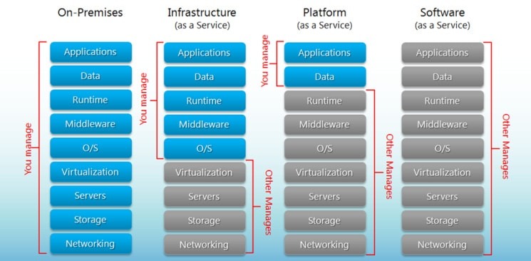
SaaS
Software as a Service
Cloud-based service providers offer end-user applications. Google Apps, DropBox, Slack, etc.
- Web access to Software (primarily commercial).
- Software is managed from a central location.
- Delivery 1 - many models.
- No patches, No upgrades
When not to use
- Hardware integration is needed. (Price Scanner)
- Faster processing is required.
- Cannot host data outside the premise.
PaaS
Platform as a Service
Software tools are available over the internet. AWS RDS, Heroku, Salesforce
- Scalable
- Built on Virtualization Technology
- No User needed to maintain software. (DB upgrades, patches by cloud team)
When not to use PaaS
- Propriety tools don't allow moving to diff providers. (AWS-specific tools)
- Using new software that is not part of the PaaS toolset.
IaaS
Infrastructure as a Service
Cloud-based hardware services. Pay-as-you-go services for Storage, Networking, and Servers.
Amazon EC2, Google Compute Engine, S3.
- Highly flexible and scalable.
- Accessible by more than one user.
- Cost-effective (if used right).
Serverless computing
Focuses on building apps without spending time managing servers/infrastructure.
Feature automatic scaling, built-in high availability, and pay-per-use.
Use of resources when a specific function or event occurs.
Cloud providers handle the deployment, and capacity, and manage the servers.
Example: AWS Lambda, AWS Step Functions.
Easy way to remember SaaS, PaaS, IaaS
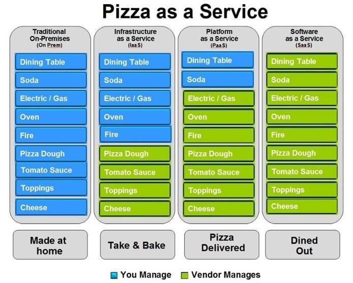
bigcommerce.com
Challenges of Cloud Computing
Privacy: "Both traditional and Big Data sets often contain sensitive information, such as addresses, credit card details, or social security numbers."
So, it's the responsibility of users to ensure proper security methods are followed.
Compliance: Cloud providers replicate data across regions to ensure safety. If companies have regulations that data should not be stored outside their organization or should not be stored in a specific part of the world.
Data Availability: Everything is dependent on the Internet and speed. It is also dependent on the choice of the cloud provider. Big companies like AWS / GCP / Azure have more data centers and backup facilities.
Connectivity: Internet availability + speed.
Vendor lock-in: Once an organization has migrated its data and applications to the cloud, switching to a different provider can be difficult and expensive. This is known as vendor lock-in. Some cloud agnostic tools like Databricks help enterprises to mitigate this problem, but still, its a challenge.
Cost: Cloud computing can be a cost-effective way to deploy and manage IT resources. However, it is essential to carefully consider your needs and budget before choosing a cloud provider.
Continuous Training: Employees may need to be trained to use cloud-based applications. This can be a cost and time investment.
Constant Change in Technology: Cloud providers constantly improve or change their technology. Recently, Microsoft decided to decommission Synapse and launch a new tool called Fabric.
AWS
Terms to Know
Elasticity The ability to acquire resources as you need them and release resources when you no longer need them.
Scale Up vs. Scale Down
Scale-Out vs. Scale In
Latency
Typically latency is a measurement of a round-trip between two systems, such as how long it takes data to make its way between two.
Root User
Owner of the AWS account.
IAM
Identity Access Management
ARN
Amazon Resource Name
For example
arn:aws:iam::123456789012:user/Development/product_1234/*
Policy
Rules
AWS Popular Services
Amazon EC2
Allows you to deploy virtual servers within your AWS environment.
Amazon VPC
An isolated segment of the AWS cloud accessible by your own AWS account.
Amazon S3
A fully managed, object-based storage service that is highly available, highly durable, cost-effective, and widely accessible.
AWS IAM (Identify and Access Mgt)
Used to manage permissions to your AWS resources
AWS Management Services
Amazon EC2 Auto Scaling
Automatically increases or decreases your EC2 resources to meet the demand based on custom-defined metrics and thresholds.
Amazon CloudWatch
A comprehensive monitoring tool allows you to monitor your services and applications in the cloud.
Elastic Load Balancing
Used to manage and control the flow of inbound requests to a group of targets by distributing these requests evenly across a targeted resource group.
Billing & Budgeting
Helps control the cost.
AWS Global Infrastructure
The Primary two items are given below.
- Availability Zones
- Regions
Availability Zones (AZs)
AZs are the physical data centers of AWS.
This is where the actual computing, storage, network, and database resources are hosted that we as consumers, provision within our Virtual Private Clouds (VPCs).
A common misconception is that a single availability zone equals a single data center. Multiple data centers located closely form a single availability zone.
Each AZ will have another AZ in the same geographical area. Each AZ will be isolated from others using a separate power/network like DR.
Many AWS services use low latency links between AZs to replicate data for high availability and resilience purposes.
Multiple AZs are defined as an AWS Regions. (Example: Virginia)
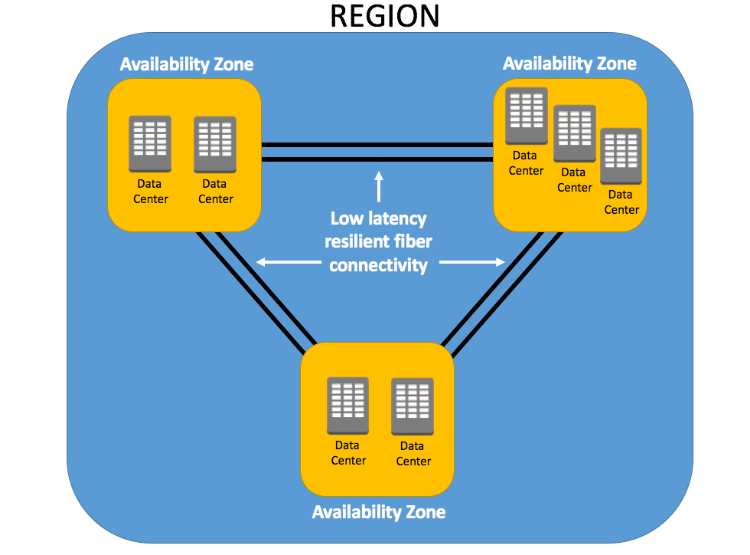
Regions
Every Region will act independently of the others, containing at least two Availability Zones.
Interestingly, only some AWS services are available in some regions.
- US East (N. Virginia) us-east-1
- US East (Ohio) us-east-2
- EU (Ireland) eu-west-1
- EU (Frankfurt) eu-central-1
Note: As of today, AWS is available in 27 regions and 87 AZs
https://docs.aws.amazon.com/AmazonRDS/latest/UserGuide/Concepts.RegionsAndAvailabilityZones.html"
EC2
(Elastic Cloud Compute)
Compute: Closely related to CPU/RAM
Elastic Compute Cloud (EC2): AWS EC2 provides resizable compute capacity in the cloud, allowing you to run virtual servers as per your needs.
Instance Types: EC2 offers various instance types optimized for different use cases, such as general purpose, compute-optimized, memory-optimized, and GPU instances.
Pricing Models
On-Demand: Pay for computing capacity by the hour or second.
Reserved: Commit to a one or 3-year term and get a discount.
Spot: Bid for unused EC2 capacity at a reduced cost.
Savings Plans: Commit to consistent compute usage for lower prices. AMI (Amazon Machine Image): Pre-configured templates for your EC2 instances, including the operating system, application server, and applications.
Security
Security Groups: Act as a virtual firewall for your instances to control inbound and outbound traffic.
Key Pairs: These are used to access your EC2 instances via SSH or RDP securely.
Elastic IPs: These are static IP addresses that can be associated with EC2 instances. They are useful for hosting services that require a consistent IP.
Auto Scaling: Automatically adjusts the number of EC2 instances in response to changing demand, ensuring you only pay for what you need.
Elastic Load Balancing (ELB): Distributes incoming traffic across multiple EC2 instances, improving fault tolerance and availability.
EBS (Elastic Block Store): Provides persistent block storage volumes for EC2 instances, allowing data to be stored even after an instance is terminated.
Regions and Availability Zones: EC2 instances can be deployed in various geographic regions, each with multiple availability zones for high availability and fault tolerance.
Storage
Persistent Storage
- Elastic Block Storage (EBS) Volumes / Logically attached via AWS network.
- Automatically replicated.
- Encryption is available.
Ephemeral Storage - Local storage
- Physically attached to the underlying host.
- When the instance is stopped or terminated, all the data is lost.
- Rebooting will keep the data intact.
DEMO - Deploy EC2
S3
(Simple Storage Service)
It's an IaaS service.
- Highly Available
- Durable
- Cost Effective
- Widely Accessible
- Uptime of 99.99%
-
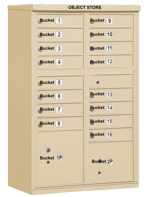
Objects and Buckets: The fundamental elements of Amazon S3 are objects and buckets. Objects are the individual data pieces stored in Amazon S3, while buckets are containers for these objects. An object consists of a file and, optionally, any metadata that describes that file.
-
It's also a regional service, meaning that when you create a bucket, you specify a region, and all objects are stored there.
-
Globally Unique: The name of an Amazon S3 bucket must be unique across all of Amazon S3, that is, across all AWS customers. It's like a domain name.
-
Globally Accessible: Even though you specify a particular region when you create a bucket, once the bucket is created, you can access it from anywhere in the world using the appropriate URL.
-
-
Scalability: Amazon S3 can scale in terms of storage, request rate, and users to support unlimited web-scale applications.
-
Security: Amazon S3 includes several robust security features, such as encryption for data at rest and in transit, access controls like Identity and Access Management (IAM) policies, bucket policies, and Access Control Lists (ACLs), and features for monitoring and logging activity, like AWS CloudTrail.
-
Data transfer: Amazon S3 supports transfer acceleration, which speeds up uploads and downloads of large objects.
-
Event Notification: S3 can notify you of specific events in your bucket. For instance, you could set up a notification to alert you when an object is deleted from your bucket.
-
Management Features: S3 has a suite of features to help manage your data, including lifecycle management, which allows you to define rules for moving or expiring objects, versioning to keep multiple versions of an object in the same bucket, and analytics for understanding and optimizing storage costs.
-
Consistency: Amazon S3 provides read-after-write consistency for PUTS of new objects and eventual consistency for overwrite PUTS and DELETES.
-
Read-after-write Consistency for PUTS of New Objects: When a new object is uploaded (PUT) into an Amazon S3 bucket, it's immediately accessible for read (GET) operations. This is known as read-after-write consistency. You can immediately retrieve a new object as soon as you create it. This applies across all regions in AWS, and it's crucial when immediate, accurate data retrieval is required.
-
Eventual Consistency for Overwrite PUTS and DELETES: Overwrite PUTS and DELETES refer to operations where an existing object is updated (an overwrite PUT) or removed (a DELETE). For these operations, Amazon S3 provides eventual consistency. If you update or delete an object and immediately attempt to read or delete it, you might still get the old version or find it there (in the case of a DELETE) for a short period. This state of affairs is temporary, and shortly after the update or deletion, you'll see the new version or find the object gone, as expected.
-
Src: Mailbox
Src: USPS
Notes
Data is stored as an "Object."
Object storage, also known as object-based storage, manages data as objects. Each object includes the data, associated metadata, and a globally unique identifier.
Unlike file storage, there are no folders or directories in object storage. Instead, objects are organized into a flat address space, called a bucket in Amazon S3's terminology.
The unique identifier allows an object to be retrieved without needing to know the physical location of the data. Metadata can be customized, making object storage incredibly flexible.
Every object gets a UID (universal ID) and associated META data.
No Folders / SubFolders
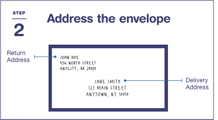
For example, if you have an object with the key images/summer/beach.png in your bucket, Amazon S3 has no internal concept of the images or summer as separate entities—it simply sees the entire string images/summer/beach.png as the key for that object.
To store objects in S3, you must first define and create a bucket.
You can think of a bucket as a container for your data.
This bucket name must be unique, not just within the region you specify, but globally against all other S3 buckets, of which there are many millions.
Any object uploaded to your buckets is given a unique object key to identify it.
- S3 bucket ownership is not transferable.
- S3 bucket names should start with alphabets, and - is allowed in between.
- An AWS account can have a maximum of 100 buckets.
More details
https://docs.aws.amazon.com/AmazonS3/latest/userguide/object-keys.html
Other types of Storage are
File Storage
Block Storage
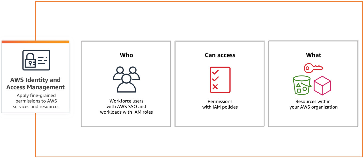
description: Identity Access Management
IAM
src: Aws
ARN: Amazon Resource Name
Users - Individual Person / Application
Groups - Collection of IAM Users
Policies - Policy sets permission/control access to AWS resources. Policies are stored in AWS as JSON documents.
A Policy can be attached to multiple entities (users, groups, and roles) in your AWS account.
Multiple Policies can be created and attached to the user.
Roles - Set of permissions that define what actions are allowed and denied by an entity in the AWS console. Similar to a user, it can be accessed by any type of entity.
// Examples of ARNs

arn:aws:s3:::my_corporate_bucket/*

arn:aws:s3:::my_corporate_bucket/Development/*

arn:aws:iam::123456789012:user/chandr34

arn:aws:iam::123456789012:group/bigdataclass

arn:aws:iam::123456789012:group/*
Types of Policies
Identity-based policies: Identity-based policies are attached to an IAM user, group, or role (identities). These policies control what actions an identity can perform, on which resources, and under what conditions.
Resource-based policies: Resource-based policies are attached to a resource such as an Amazon S3 bucket. These policies control what actions a specified principal can perform on that resource and under what conditions.
Permission Boundary: You can use an AWS-managed policy or a customer-managed policy to set the boundary for an IAM entity (user or role). A permissions boundary is an advanced feature for using a managed policy to set the maximum permissions that an identity-based policy can grant to an IAM entity.
Inline Policies: Policies that are embedded in an IAM identity. Inline policies maintain a strict one-to-one relationship between a policy and an identity. They are deleted when you delete the identity.
AWS CloudShell
AWS CloudShell is a browser-based shell environment available directly through the AWS Management Console. It provides a command-line interface (CLI) to manage and interact with AWS resources securely without needing to install any software or set up credentials on your local machine.
Use Cases
Quick Access to AWS CLI
Allows you to run AWS CLI commands directly without configuring your local machine. It's perfect for quick tasks like managing AWS resources (e.g., EC2 instances, S3 buckets, or Lambda functions).
Development and Automation
You can write and execute scripts using common programming languages like Python and Shell. It’s great for testing and automating tasks directly within your AWS environment.
Secure and Pre-Configured Environment
AWS CloudShell comes pre-configured with AWS CLI, Python, Node.js, and other essential tools. It uses your IAM permissions, so you don’t need to handle keys or credentials directly, making it secure and convenient.
Access to Filesystem and Persistent Storage
You get a persistent 1 GB home directory per region to store scripts, logs, or other files between sessions, which can be used to manage files related to your AWS resources.
Cross-Region Management
You can access and manage resources across different AWS regions directly from CloudShell, making it useful for multi-region setups.
Basic Commands
    aws s3 ls
    aws ec2 describe-instances

    sudo apt install jq
list_buckets.sh
#!/bin/bash
echo "Listing all S3 buckets:"
aws s3 ls
bash list_buckets.sh
# get account details

aws sts get-caller-identity

# list available regions

aws ec2 describe-regions --query "Regions[].RegionName" --output table

# create a bucket

aws s3 mb s3://chandr34-newbucket

# upload a file to a bucket

echo "Hello, CloudShell!" > hello.txt
aws s3 cp hello.txt s3://chandr34-newbucket

# List files in bucket

aws s3 ls s3://chandr34-newbucket/

# Delete bucket  with files

aws s3 rb s3://chandr34-newbucket --force

# List AMIs

aws ec2 describe-images --owners amazon --query 'Images[*].{ID:ImageId,Name:Name}' --output table

# quickly launch a ec2

aws ec2 create-key-pair --key-name gcnewkeypair --query 'KeyMaterial' --output text > myNewKeyPair.pem

# Change Permission

chmod 0400 myNewKeyPair.pem

# Launch new EC2

aws ec2 run-instances --image-id ami-0866a3c8686eaeeba --count 1 --instance-type t2.micro --key-name gcnewkeypair --security-groups default

# Get Public IP

aws ec2 describe-instances --query "Reservations[].Instances[].PublicIpAddress" --output text

# Login to server

ssh -i myKeyNewPair.pem ubuntu@<getthehostip>

# terminate the instance

aws ec2 terminate-instances --instance-ids <>
Cloud Formation
my-webserver.yml
AWSTemplateFormatVersion: '2010-09-09'
Description: CloudFormation template to launch an Amazon Linux EC2 instance with Nginx installed.

Resources:
  MyEC2Instance:
    Type: AWS::EC2::Instance
    Properties:
      InstanceType: t2.micro
      ImageId: ami-0866a3c8686eaeeba
      KeyName: gcnewkeypair
      SecurityGroupIds:
        - !Ref InstanceSecurityGroup
      UserData:
        Fn::Base64:
          !Sub |
            #!/bin/bash
            apt update -y
            apt install -y nginx
            systemctl start nginx
            systemctl enable nginx
      Tags:
        - Key: Name
          Value: MyNginxServer

  InstanceSecurityGroup:
    Type: AWS::EC2::SecurityGroup
    Properties:
      GroupDescription: Enable SSH and HTTP access
      SecurityGroupIngress:
        - IpProtocol: tcp
          FromPort: 22
          ToPort: 22
          CidrIp: 0.0.0.0/0  # SSH access, restrict this to your IP range for security
        - IpProtocol: tcp
          FromPort: 80
          ToPort: 80
          FromPort: 443
          ToPort: 443
          CidrIp: 0.0.0.0/0  # HTTP access for Nginx

Outputs:
  InstanceId:
    Description: The Instance ID of the EC2 instance
    Value: !Ref MyEC2Instance
  PublicIP:
    Description: The Public IP address of the EC2 instance
    Value: !GetAtt MyEC2Instance.PublicIp
  WebURL:
    Description: URL to access the Nginx web server
    Value: !Sub "http://${MyEC2Instance.PublicIp}"
Launch the Stack via CloudShell
# Create the stack
aws cloudformation create-stack --stack-name gc-stack --template-body file://my-webserver.yml --capabilities CAPABILITY_NAMED_IAM


# Check the status

aws cloudformation describe-stacks --stack-name gc-stack --query "Stacks[0].StackStatus"


aws cloudformation describe-stacks --stack-name gc-stack --query "Stacks[0].Outputs"

# delete the stack

aws cloudformation delete-stack --stack-name gc-stack


aws cloudformation describe-stacks --stack-name gc-stack --query "Stacks[0].StackStatus"

# confirm the deletion status

aws cloudformation list-stacks --query "StackSummaries[?StackName=='gc-stack'].StackStatus"
Terraform
Features of Terraform
Infrastructure as Code: Terraform allows you to write, plan, and create infrastructure using configuration files. This makes infrastructure management automated, consistent, and easy to collaborate on.
Multi-Cloud Support: Terraform supports many cloud providers and on-premises environments, allowing you to manage resources across different platforms seamlessly.
State Management: Terraform keeps track of the current state of your infrastructure in a state file. This enables you to manage changes, plan updates, and maintain consistency in your infrastructure.
Resource Graph: Terraform builds a resource dependency graph that helps in efficiently creating or modifying resources in parallel, speeding up the provisioning process and ensuring dependencies are handled correctly.
Immutable Infrastructure: Terraform promotes the practice of immutable infrastructure, meaning that resources are replaced rather than updated directly. This ensures consistency and reduces configuration drift.
Execution Plan: Terraform provides an execution plan (terraform plan) that previews changes before they are applied, allowing you to understand and validate the impact of changes before implementing them.
Modules: Terraform supports reusability through modules, which are self-contained, reusable pieces of configuration that help you maintain best practices and reduce redundancy in your infrastructure code.
Community and Ecosystem: Terraform has a large open-source community and many providers and modules available through the Terraform Registry, which makes it easier to get started and integrate with various services.
Use Cases
- Multi-Cloud Provisioning
- Infrastructure Scaling
- Disaster Recovery
- Environment Management
- Compliance & Standardization
- CI/CD Pipelines
- Speed and Simplicity
- Team Collaboration
- Error Reduction
- Enhanced Security
Install Terraform CLI
Terraform Structure
Provider Block: Specifies the cloud provider or service (e.g., AWS, Azure, Google Cloud) that Terraform will interact with.
provider "aws" {
  region = "us-east-1"
}
Resource Block: Defines the resources to be created or managed. A resource can be a server, network, or other infrastructure component.
resource "aws_instance" "example" {
  ami           = "ami-0c55b159cbfafe1f0"
  instance_type = "t2.micro"
}
Data Block: Fetches information about existing resources, often for referencing in resource blocks.
data "aws_ami" "latest" {
  most_recent = true
  owners      = ["amazon"]
}
Variable Block: Declares input variables to make the script flexible and reusable.
variable "instance_type" {
  description = "Type of instance to use"
  type        = string
  default     = "t2.micro"
}
Output Block: Specifies values to be output after the infrastructure is applied, like resource IDs or connection strings.
output "instance_ip" {
  value = aws_instance.example.public_ip
}
Module Block: Used to encapsulate and reuse sets of Terraform resources.
module "vpc" {
  source = "./modules/vpc"
  cidr_block = "10.0.0.0/16"
}
Locals Block: Defines local values that can be reused in the configuration.
locals {
  environment = "production"
  instance_count = 3
}
SET these environment variables.
export AWS_ACCESS_KEY_ID="your-access-key-id"
export AWS_SECRET_ACCESS_KEY="your-secret-access-key"
Simple S3 Bucket
simple_s3_bucket.tf
terraform {
  required_providers {
    aws = {
      source  = "hashicorp/aws"
      version = "~> 5.70.0"
    }
  }

  required_version = ">= 1.2.0"
}

provider "aws" {
  region = "us-east-1"
  profile = "chandr34"
}

resource "aws_s3_bucket" "demo" {
  bucket = "chandr34-my-new-tf-bucket"

  tags = {
    Createdusing = "tf"
    Environment  = "classdemo"
  }
}

output "bucket_name" {
  value = aws_s3_bucket.demo.bucket
}
Create a new folder
Copy the .tf into it
terraform init
terraform validate
terraform plan
terraform apply
terraform destroy
Variable S3 Bucket
variable_bucket.tf
terraform {
  required_providers {
    aws = {
      source  = "hashicorp/aws"
      version = "~> 5.70.0"
    }
  }

  required_version = ">= 1.2.0"
}

provider "aws" {
  region  = "us-east-1"
  profile = "chandr34"
}

variable "bucket_name" {
  description = "The name of the S3 bucket to create"
  type        = string
}

resource "aws_s3_bucket" "demo" {
  bucket = var.bucket_name

  tags = {
    Createdusing = "tf"
    Environment  = "classdemo"
  }
}

output "bucket_name" {
  value = aws_s3_bucket.demo.bucket
}
Create a new folder
Copy the .tf into it
terraform init
terraform validate
terraform plan
terraform apply -var="bucket_name=chandr34-variable-bucket"
terraform destroy -var="bucket_name=chandr34-variable-bucket"
Variable file
Any filename with extension .tfvars
terraform.tfvars
bucket_name = "chandr34-variable-bucket1"
terraform apply -auto-approve
Please make sure AWS Profile is created.
Create Public and Private Keys
Linux / Mac Users
// create private/public key

ssh-keygen -b 2048 -t rsa -f ec2_tf_demo
Windows Users
Open PuttyGen and create a Key
Terraform
- mkdir simple_ec2
- cd tf-aws-ec2-sample
- Create main.tf
// main.tf
#https://registry.terraform.io/providers/hashicorp/aws/latest

terraform {
  required_providers {
    aws = {
      source  = "hashicorp/aws"
      version = "~> 5.70.0"
    }
  }

  required_version = ">= 1.2.0"
}

provider "aws" {
  region  = "us-east-1"
  profile = "chandr34"
}

resource "aws_key_pair" "generated_key" {
  key_name   = "generated-key-pair"
  public_key = tls_private_key.generated_key.public_key_openssh
}

resource "tls_private_key" "generated_key" {
  algorithm = "RSA"
  rsa_bits  = 2048
}

resource "local_file" "private_key_file" {
  content  = tls_private_key.generated_key.private_key_pem
  filename = "${path.module}/generated-key.pem"
}

resource "aws_instance" "ubuntu_ec2" {
  ami           = "ami-00874d747dde814fa"
  instance_type = "t2.micro"
  key_name      = aws_key_pair.generated_key.key_name
  vpc_security_group_ids = [aws_security_group.ec2_security_group.id]

  tags = {
    Name        = "UbuntuInstance"
    Environment = "classdemo"
  }
}

resource "aws_security_group" "ec2_security_group" {
  name        = "ec2_security_group"
  description = "Allow SSH and HTTP access"

  ingress {
    from_port   = 22
    to_port     = 22
    protocol    = "tcp"
    cidr_blocks = ["0.0.0.0/0"]  # Allow SSH from anywhere (use cautiously)
  }

  ingress {
    from_port   = 80
    to_port     = 80
    protocol    = "tcp"
    cidr_blocks = ["0.0.0.0/0"]  # Allow HTTP from anywhere
  }

  egress {
    from_port   = 0
    to_port     = 0
    protocol    = "-1"
    cidr_blocks = ["0.0.0.0/0"]  # Allow all outbound traffic
  }

  tags = {
    Name = "EC2SecurityGroup"
  }
}

output "ec2_instance_public_ip" {
  value = aws_instance.ubuntu_ec2.public_ip
}

output "private_key_pem" {
  value     = tls_private_key.generated_key.private_key_pem
  sensitive = true
}
goto terminal
- terraform init
- terraform fmt
- terraform validate
- terraform apply
- terraform show
Finally
- terraform destroy
Data Architecture
- Medallion Architecture
- Bronze to Silver
- Silver to Gold
- Sample Data from Raw to Silver]
- Spark Intro
- Delta
Medallion Architecture
Medallion architecture is a data design pattern commonly used in modern data lakes and data warehouses, particularly in cloud-based environments.
A medallion architecture is a data design pattern used to logically organize data in a lakehouse, aiming to incrementally and progressively improve the structure and quality of data as it flows through each layer of the architecture (from Bronze ⇒ Silver ⇒ Gold layer tables).
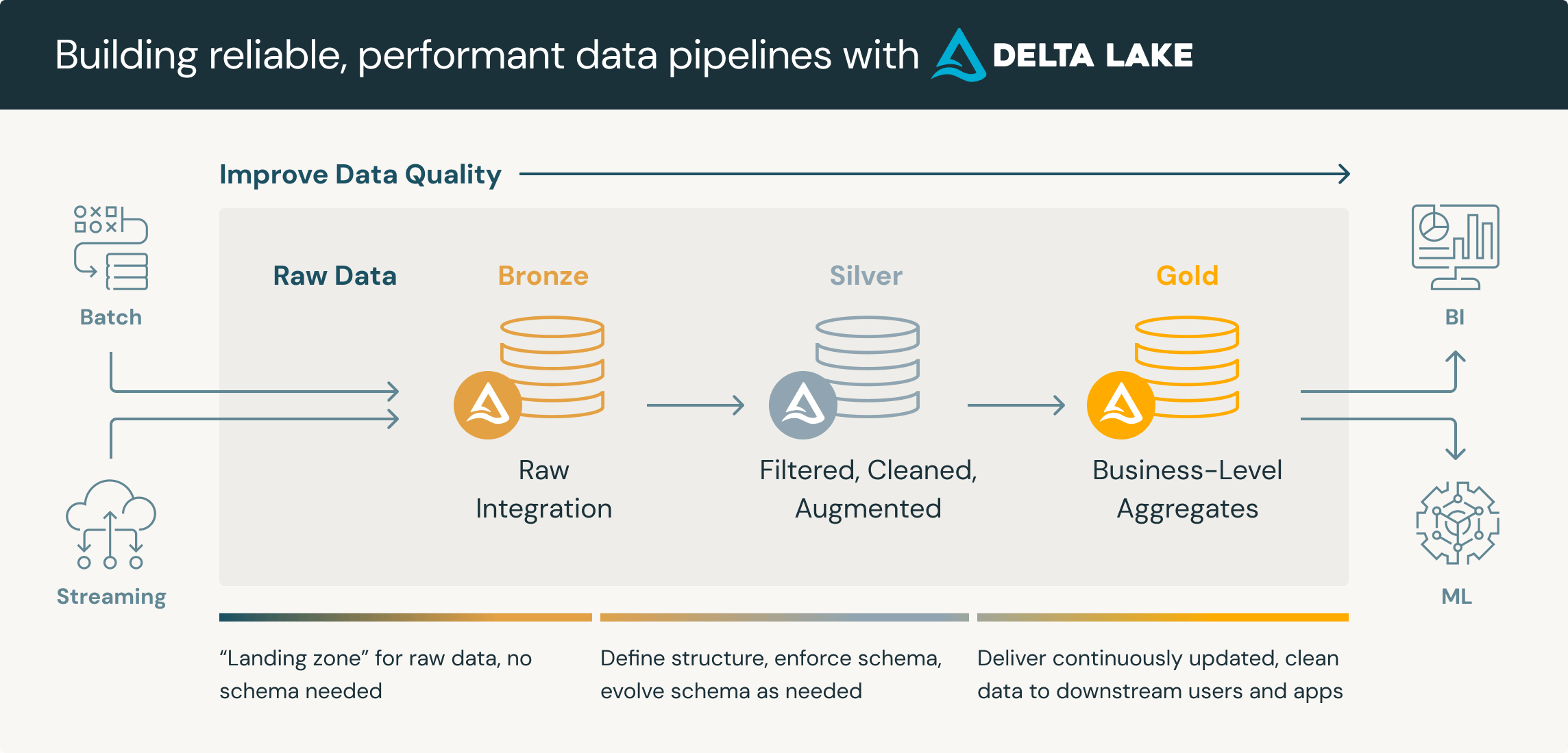
The Three Tiers
Bronze (Raw)
- Contains raw, unprocessed data.
- Typically a 1:1 copy of source system data.
- Preserves the original data for auditability and reprocessing if needed.
- Often stored in formats like JSON, CSV, or Avro.
Silver (Cleaned and Conformed)
- Cleansed and conformed version of bronze data.
- Applies data quality rules, handles missing values, deduplication.
- Often includes parsed and enriched data.
- Typically stored in a more optimized format like Parquet or Delta.
Gold (Business-Level)
- Contains highly refined, query-ready data sets.
- Often aggregated and joined from multiple silver tables.
- Optimized for specific business domains or use cases.
- Can include star schemas, data marts, or wide denormalized tables.
Key Principles
- Data flows from Bronze → Silver → Gold
- Each tier adds value and improves data quality
- Promotes data governance and lineage tracking
- Enables self-service analytics at different levels of refinement
Benefits
Flexibility: Supports various data processing needs
Scalability: Easily accommodates growing data volumes
Governance: Improves data lineage and auditability
Performance: Optimizes query performance on refined data sets
Reusability: Allows multiple downstream applications to use appropriately refined data
Bronze to Silver
These are the basic best practices followed when moving data from Bronze to Silver.
DO's
Case standardization
- Convert column names to lowercase or uppercase.
- Standardize text fields (e.g., convert all First Name, Last Name, Product names to title case).
Column renaming
- Adopt consistent naming conventions across tables
Whitespace
- Trim leading and trailing spaces from string fields.
- Remove extra spaces between words.
Data type conversions
- Convert string dates to proper date format
- Change numeric strings to appropriate integer or decimal types
Null handling
- Replace empty strings with NULL values
- Set default values for NULL fields where appropriate
Deduplication
- Remove exact duplicate records
- Handle near-duplicates based on business rules
Format standardization
- Normalize phone numbers to a consistent format
- Standardize address formats
Value normalization
- Convert units of measurement to a standard unit (e.g., all weights to pounds or kgs)
- Standardize currency / lat-long decimal positions.
Character encoding
- Convert all text to UTF-8 or another standard encoding.
Special character handling
- Remove or replace non-printable characters.
- Handle escape characters in text fields.
Data validation
- Check for values within expected ranges
- Validate against reference data (e.g., valid product codes)
Date and time standardization
- Convert all timestamps to UTC or a standard time zone
- Ensure consistent date formats across all fields
Calculated fields
- Add derived columns based on raw data (e.g., age from birth date)
Data enrichment
- Add geographic information based on zip codes
- Categorize products based on attributes
Error correction
- Fix common misspellings
- Correct known data entry errors
Structural changes:
- Split combined fields (e.g., full name into first and last name).
- Merge related fields for easier analysis.
Metadata addition:
- Add source system identifiers.
- Include data lineage information.
Sensitive data handling
- Mask or encrypt personally identifiable information (PII)
- Apply data governance rules
Outlier detection and handling
- Identify statistical outliers
- Apply business rules to handle extreme values
Column dropping
- Remove unnecessary or redundant columns
DON'Ts
Don't Lose Raw Data
- Avoid modifying or transforming data in a way that the original information is lost. Always keep the Bronze layer intact and unmodified as it serves as the source of truth.
- Maintain backups of critical data and metadata in case you need to revert transformations.
Don't Over-optimize Early
- Avoid excessive transformations or optimizations before ensuring data accuracy.
- Focus on clarity and correctness before performance tuning.
Don't Hard-code Business Logic
- Avoid hard-coding business rules that could change frequently. Instead, make them configurable to ensure flexibility for future updates.
Don't Skip Data Validation
- Don’t blindly trust incoming data from the Bronze layer. Always validate the quality, type, and range of data before moving it to Silver.
- Implement rules for handling invalid data, such as setting defaults for missing values or discarding outliers.
Don't Ignore Metadata
- Always retain important metadata, such as source system identifiers, data lineage, or event timestamps, to maintain traceability.
Don't Introduce Ambiguity
- Avoid renaming columns or values without proper documentation. Ensure that any renaming or transformation is clear, consistent, and well-documented to prevent confusion.
Don't Remove Critical Columns Without Backup
- Avoid dropping columns that might be required later for audits or debugging. Always ensure you have a backup or metadata for columns you drop.
Don't Assume Data Integrity
- Never assume that data from the Bronze layer is clean or consistent. Always apply deduplication, null handling, and data cleaning rules.
Don't Overload the Silver Layer with Business Logic
- Avoid implementing complex business rules in the Silver layer. Keep it focused on data cleansing and preparation. Reserve detailed business logic for the Gold layer.
Don't Over-transform Data
- Avoid excessive or unnecessary transformations in the Silver layer, which could make the data less flexible for future use cases.
Don't Change Granularity
- Don’t aggregate or change the granularity of data too early. Keep data at the same granularity as the Bronze layer to maintain flexibility for future aggregations in the Gold layer.
Don't Overlook Data Encoding and Formats
- Don’t assume uniform character encoding across all systems. Always validate encoding, such as converting text to UTF-8 where needed.
- Standardize date formats and ensure consistent time zones (preferably UTC) across all fields.
Don't Disregard Null and Missing Data
- Don't ignore patterns of missing data. Treat NULL values carefully, ensuring that they’re handled based on the specific business logic.
Don't Apply Unnecessary Joins
- Avoid applying joins that aren’t required in the Silver layer. Unnecessary joins can increase complexity and lead to performance degradation.
Don't Remove Contextual Information
- Don’t drop fields that provide necessary context, such as event timestamps, source system details, or audit trails.
Don't Assume All Data Sources Are Consistent
- Don’t assume that data from different sources (even within the Bronze layer) will have consistent formats, structures, or units of measurement. Always validate and normalize data as necessary.
Don't Ignore Data Governance
- Avoid handling sensitive data like PII carelessly. Ensure that you apply data masking, encryption, or other governance rules to stay compliant with regulations.
Don't Forget Documentation
- Avoid performing transformations or renaming columns without thoroughly documenting them. Clear documentation ensures data transformations are transparent and easily understood across teams.
Silver to Gold
These are the basic best practices followed when moving data from Silver to Gold.
Business alignment
- Tailor Gold datasets to specific business needs and use cases
- Collaborate closely with business stakeholders to understand requirements
Aggregation and summarization
- Create pre-aggregated tables for common metrics (e.g., daily sales totals)
- Implement various levels of granularity to support different analysis needs
Dimensional modeling
- Develop star or snowflake schemas for analytical queries
- Create conformed dimensions for consistent reporting across the organization
Denormalization
- Create wide, denormalized tables for specific reporting needs
- Balance performance gains against data redundancy
Metric standardization
- Implement agreed-upon business logic for key performance indicators (KPIs)
- Ensure consistent calculation of metrics across different Gold datasets
Data mart creation
- Develop subject-area specific data marts (e.g., Sales, HR, Finance)
- Optimize each mart for its intended use case
Advanced transformations
- Apply complex business rules and calculations
- Implement time-based analyses (e.g., year-over-year comparisons)
Data quality assurance
- Implement rigorous testing of Gold datasets
- Set up automated data quality checks and alerts
Performance optimization
- Use appropriate indexing and partitioning strategies
- Implement materialized views for frequently accessed data
Metadata management
- Maintain detailed business glossaries and data dictionaries
- Document data lineage and transformation logic
Access control
- Implement fine-grained access controls for sensitive data
- Ensure compliance with data governance policies
Versioning and historization
- Implement slowly changing dimensions (SCDs) where appropriate
- Maintain historical versions of key business entities
Data freshness
- Define and implement appropriate refresh schedules
- Balance data currency against processing costs
Self-service enablement
- Create views or semantic layers for business users
- Provide clear documentation and training for end-users
Caching strategies
- Implement intelligent caching for frequently accessed data
- Balance cache freshness against query performance
Query optimization
- Tune common queries for optimal performance
- Create aggregated tables or materialized views for complex calculations
Data exploration support:
- Provide sample queries or analysis templates
- Create dashboards or reports showcasing the value of Gold datasets
Scalability considerations
- Design Gold datasets to handle growing data volumes
- Implement appropriate archiving strategies for historical data
Documentation
- Maintain comprehensive documentation of Gold dataset structures and uses
- Provide clear guidelines on how to use and interpret the data
Sample Data from Raw to Silver
Using DUCKDB
Raw CSV : Sales_100
Creating Bronze
create table bronze_sales as select * from read_csv("https://raw.githubusercontent.com/gchandra10/filestorage/refs/heads/main/sales_100.csv");
Creating Silver
CREATE SEQUENCE sales_id_seq;

CREATE TABLE silver_sales (
    id INTEGER PRIMARY KEY DEFAULT nextval('sales_id_seq'),
    region VARCHAR,
    country VARCHAR,
    item_type VARCHAR,
    sales_channel VARCHAR,
    order_priority VARCHAR,
    order_date DATE,
    order_id BIGINT,
    ship_date DATE,
    units_sold BIGINT,
    unit_price DOUBLE,
    unit_cost DOUBLE,
    total_revenue DOUBLE,
    total_cost DOUBLE,
    total_profit DOUBLE
);
Bronze Data
select distinct("Order Priority") from bronze_sales;
select distinct("Sales Channel") from bronze_sales;

insert into silver_sales(region,
country,
item_type,
sales_channel,
order_priority,
order_date,
order_id,
ship_date,
units_sold,
unit_price,
unit_cost,
total_revenue,
total_cost,
total_profit
)
select distinct * from bronze_sales where "order id" is not null;
Apache Spark
Apache Spark is a in memory - distributed data analytics engine. It is a unified engine for big data processing. Unified means it offers both batch and stream processing.
Apache Spark overcame the challenges of Hadoop with in-memory parallelization and delivering high performance for distributed processing.
Increase developer productivity and can be seamlessly combined to create complex workflows.
Features of Apache Spark
- Analytics and Big Data processing.
- Machine learning capabilities.
- Huge open source community and contributors.
- A distributed framework for general-purpose data processing.
- Support for Java, Scala, Python, R, and SQL.
- Integration with libraries for streaming and graph operations.
Benefits of Apache Spark
- Speed (In memory cluster computing)
- Scalable (Cluster can be added/removed)
- Powerful Caching
- Real-time
- Supports Delta
- Polyglot (Knowing/Using several languages. Spark provides high-level APIs in SQL/Scala/Python/R. Spark code can be written in any of these 4 languages.)
Spark Popular Eco System (Core APIs)
- Spark SQL : SQL queries in Spark.
- Streaming : Process realtime data.
- MLib : MLlib allows for preprocessing, munging, training of models, and making predictions at scale on data.
Also it supports Scala, Python, JAVA and R.
Spark Architecture
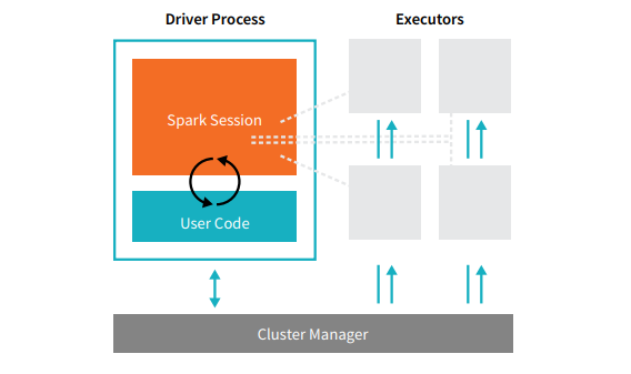
src: www.databricks.com

Cluster Manager: Allocates Students/Faculty for a course. Who is in and who is out.
Driver: Faculty point of entry. Gives instructions and collects the result.
Executor: Table of Students.
Core (Thread): Student
Cores share the same JVM, Memory, Diskspace (like students sharing table resources, power outlets)
Partition
Technique of distributing data across multiple files or nodes in order to improve the query processing performance.
By partitioning the data, you can write each partition to a different executor simultaneously, which can improve the performance of the write operation.
Spark can read each partition in parallel on a different executor, which can improve the performance of the read operation.
Bowl of candies how do sort and count by color?

If its with one person, then others are wasting their time. Instead if its packaged into small packs (partitions) then everyone can work in parallel.
Default size is 128MB and its configurable.
Data ready to be processed
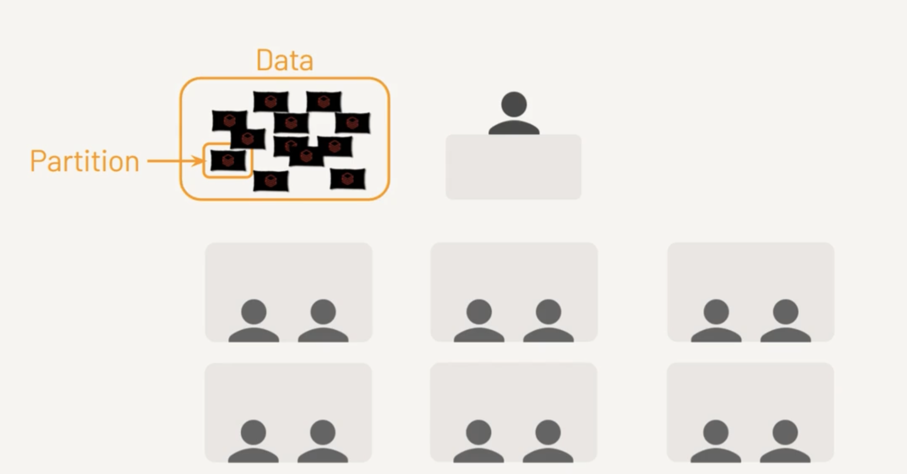
Each Core is assigned a Task

Few cores completed the Tasks

Free Cores picks up the remaining Tasks

Terms to learn
Spark Context
Used widely in Spark Version 1.x
Spark Context : Used by Driver node to establish communication with Cluster. SparkContext is an object that represents the entry point to the underlying Spark cluster, which is responsible for coordinating the processing of distributed data in a cluster. It serves as a communication channel between the driver program and the Spark cluster.
When a Databricks cluster is started, a SparkContext is automatically created and made available as the variable sc in the notebook or code. The SparkContext provides various methods to interact with the Spark cluster, including creating RDDs, accessing Spark configuration parameters, and managing Spark jobs.
text_rdd = sc.textFile("/FileStore/tables/my_text_file.txt")
Other entry points
SQL Context : Entry point to perform SQL Like operations. Hive Context : If Spark application needs to communicate with Hive.
In newer versions of Spark, this is not used anymore.
Spark Session
In Spark 2.0, we introduced SparkSession, a new entry point that subsumes SparkContext, SQLContext, StreamingContext, and HiveContext. For backward compatibiilty, they are preserved.
In short its called as "spark".
spark.read.format("csv").
RDD
RDDs (Resilient Distributed Datasets) are the fundamental data structure in Apache Spark. Here are the key aspects:
Core Characteristics:
- Resilient: Fault-tolerant with the ability to rebuild data in case of failures
- Distributed: Data is distributed across multiple nodes in a cluster
- Dataset: Collection of partitioned data elements
- Immutable: Once created, cannot be changed
Key Features:
- In-memory computing
- Lazy evaluation (transformations aren't executed until an action is called)
- Type safety at compile time
- Ability to handle structured and unstructured data
Basic Operations:
Transformations (create new RDD):
- map()
- filter()
- flatMap()
- union()
- intersection()
- distinct()
Actions (return values):
- reduce()
- collect()
- count()
- first()
- take(n)
- saveAsTextFile()
Benefits
- Fault tolerance through lineage graphs
- Parallel processing
- Caching capability for frequently accessed data
- Efficient handling of iterative algorithms
- Supports multiple languages (Python, Scala, Java)
Limitations
- No built-in optimization engine
- Manual optimization required
- Limited structured data handling compared to DataFrames
- Higher memory usage due to Java serialization
Example
Read a CSV using RDD and group by Region, Country except Region=Australia
from pyspark.sql import SparkSession
from operator import add

# Initialize Spark
spark = SparkSession.builder \
    .appName("Sales Analysis RDD") \
    .getOrCreate()

sc = spark.sparkContext

# Read CSV file
rdd = sc.textFile("sales.csv")

# Extract header and data
header = rdd.first()
data_rdd = rdd.filter(lambda line: line != header)

# Transform and filter data
# Assuming CSV format: Region,Country,Sales,...
result_rdd = data_rdd \
    .map(lambda line: line.split(',')) \
    .filter(lambda x: x[0] != 'Australia') \
    .map(lambda x: ((x[0], x[1]), float(x[2]))) \
    .groupByKey() \
    .mapValues(lambda sales: sum(sales) / len(sales)) \
    .sortByKey()

# Display results
print("Region, Country, Average Sales")
for (region, country), avg_sales in result_rdd.collect():
    print(f"{region}, {country}, {avg_sales:.2f}")
Good News you don't have to write direct RDDs anymore.
Now the same using Dataframes
from pyspark.sql import SparkSession
from pyspark.sql.functions import avg

# Initialize Spark
spark = SparkSession.builder \
    .appName("Sales Analysis DataFrame") \
    .getOrCreate()

# Read CSV file
df = spark.read \
    .option("header", "true") \
    .option("inferSchema", "true") \
    .csv("sales.csv")

# Group by and calculate average sales
result_df = df.filter(df.Region != 'Australia') \
    .groupBy('Region', 'Country') \
    .agg(avg('Sales').alias('Average_Sales')) \
    .orderBy('Region', 'Country')

# Show results
result_df.show(truncate=False)
Spark Query Execution Sequence
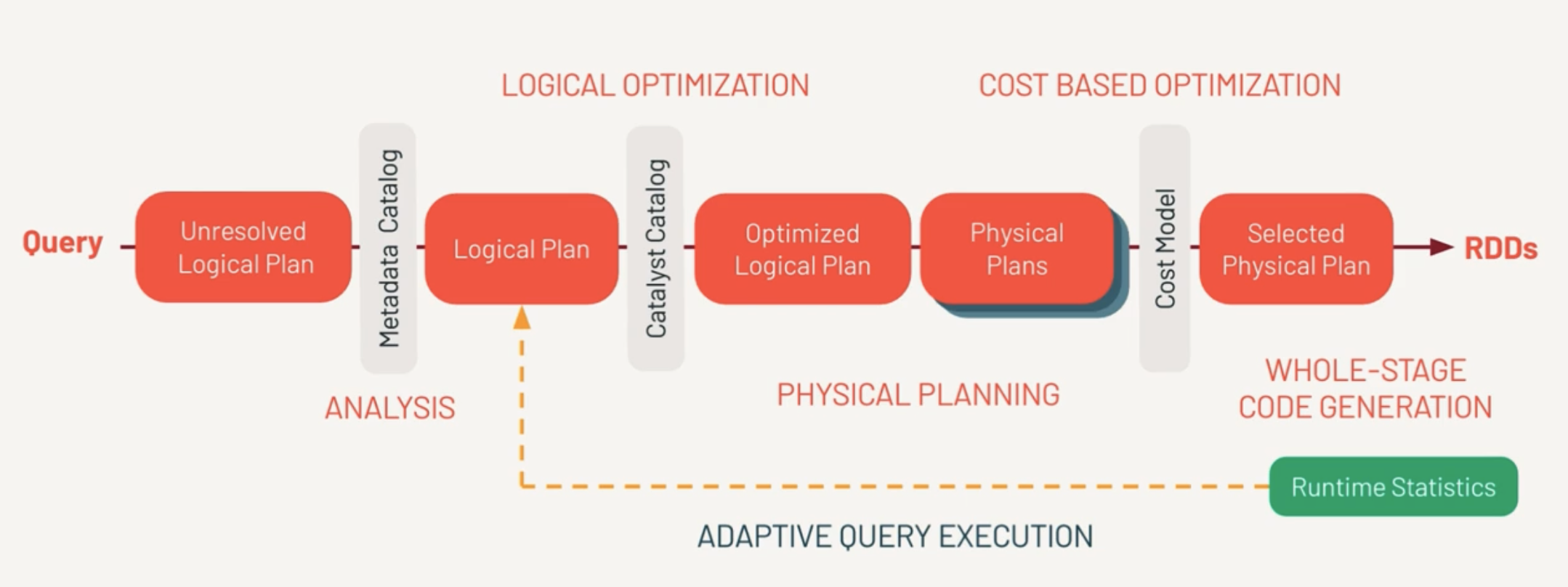
Unresolved Logical Plan
This is the set of instructions the developer logically wants to do.
First, Spark parses the query and creates the Unresolved Logical Plan Validates the syntax of the query.
Doesn’t validate the semantics meaning column name existence, data types.
Metadata Catalog (Analysis)
This is where the column names, table names are validated against Catalog and returns a Logical Plan.
Catalyst Catalog
This is where first set of optimizations takes place. Rewrite/Reorder the logical sequence of calls. From this we get Optimized Logical Plan.
Catalyst Optimizer
Determines there are multiple ways to execute the query. Do we pull 100% of data from the network or filter the dataset with a predicate pushdown? From this, we determine one or more physical plans.
Physical Plans
Multiple ways to execute the query.
Physical Plans represent what the query engine will actually do. This is different from the optimized logical plan. Each optimization determines a cost model.
Selected Physical Plan
And best performing model is selected by Cost Model. Finally the selected physical plan is compiled to RDDs.
- Estimated amount of data needed for processing
- amount of shuffling
- amount of time to execute the query
RDD
(Whole Stage Code Generation)
This the same RDD a developer would write themselves.
AQE (Adaptive Query Execution)
Checks for join strategies, skews at runtime. This happens repeatedly to find out best plan.
- explain(mode="simple") which will display the physical plan
- explain(mode="extended") which will display physical and logical plans (like “extended” option)
- explain(mode="codegen") which will display the java code planned to be executed
- explain(mode="cost") which will display the optimized logical plan and related statistics (if they exist)
- explain(mode="formatted") which will display a splitted output composed by a nice physical plan outline, and a section with each node details
DAG (Direct Acyclic Graph)
Example of DAG
Stage 1 (Read + Filter):
   [Read CSV] → [Filter]
        |
        ↓
Stage 2 (GroupBy + Shuffle):
   [Shuffle] → [GroupBy]
        |
        ↓
Stage 3 (Order):
   [Sort] → [Display]
Databricks
Databricks is a Unified Analytics Platform on top of Apache Spark that accelerates innovation by unifying data science, engineering and business. With our fully managed Spark clusters in the cloud, you can easily provision clusters with just a few clicks.
This is not Databricks Sales so not getting into roots of the product.
Open
Open standards provide easy integration with other tools plus secure, platform-independent data sharing.
Unified
One platform for your data, consistently governed and available for all your analytics and AI,
Scalable
Scale efficiently with every workload from simple data pipelines to massive LLMs.
Lakehouse
Data Warehouse + Data Lake = Lakehouse.

ELT Data Design Pattern
In ELT (Extract, Load, Transform) data design patterns, the focus is on loading raw data into a data warehouse first, and then transforming it. This is in contrast to ETL, where data is transformed before loading. ELT is often favored in cloud-native architectures.
Batch Load
In a batch load, data is collected over a specific period and then loaded into the data warehouse in one go.
Real-time Example
A retail company collects sales data throughout the day and then runs a batch load every night to update the data warehouse. Analysts use this data the next day for reporting and decision-making.
Stream Load
In stream loading, data is continuously loaded into the data warehouse as it's generated. This is useful in scenarios requiring real-time analytics and decision-making.
Real-time Example
A ride-sharing app collects GPS coordinates of all active rides. This data is streamed in real-time into the data warehouse, where it's immediately available for analytics to optimize ride allocation and pricing dynamically.
Delta
Delta Lake is an open-source storage framework that enables building a Lakehouse architecture with compute engines, including Spark, PrestoDB, Flink, Trino, and Hive, and APIs for Scala, Java, Rust, Ruby, and Python.
ACID Transactions - Protect your data with the strongest level of isolation
Time Travel - Access to earlier versions of data for audits, rollbacks, or reproduce.
Open Source - Community Driven.
DML Operations - SQL,Scala,Python APIs to merge, update and delete data.
Audit History - Delta Lake logs all changes details providing a complete audit trail.
Schema Evolution/Enforcement - Prevent bad data from causing data corruption.
Unified Batch/Streaming - Exactly once ingestion to backfill to interactive queries.
Delta table is the default data table format in Databricks.
Data Warehousing Concepts
- Dimensional Modelling
- Dimension - Fact
- Sample Excercise
- Keys
- More Examples
- Master Data Management
- Steps of Dimensional Modeling
- Types of Dimensions
- Types of Facts
- Sample Data Architecture Diagram
- Data Pipeline Models
- New DW Concepts
Dimensional Modelling
Dimensional Modeling (DM) is a data structure technique optimized for data storage in a Data warehouse. Dimensional modeling aims to optimize the database for faster data retrieval. The concept of Dimensional Modeling was developed by Ralph Kimball and consisted of "fact" and "dimension" tables.
Dimension Table
Dimension provides the context surrounding a business process event; they give who, what, and where of a fact. In the Sales business process, for the fact quarterly sales number, dimensions would be
Who – Customer Names
Where – Location
What – Product Name
They are joined to Fact tables via a foreign key.
Dimensions offer descriptive characteristics of the facts with the help of their attributes.
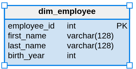
Src: www.guru99.com
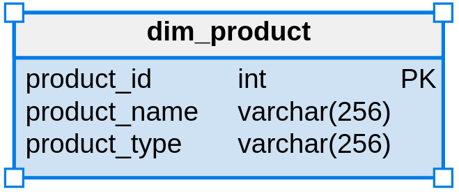
Src: www.guru99.com
Fact Table
It contains Measurements, metrics, and facts about a business process, the primary table in dimension modeling.
A Fact Table contains
Measurements/facts
Foreign key to the dimension table
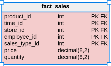
Src: www.guru99.com
Star Schema
Star schema is the simplest model used in DWH. It's commonly used in Data Marts.
Star schema is built to streamline the process.
ETL process will produce data from the operational database, transform it into the proper format, and load it into the warehouse.
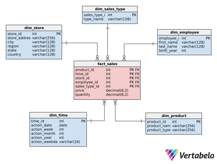
src: www.vertabelo.com
dim_employee: info about employee

dim_product: info about the product

dim_store: info about store

dim_sales_type: info about sales

dim_time: the time dimension

fact_sales: references to dimension tables plus two facts (price and quantity sold)
This Star schema is intended to store the history of placed orders.
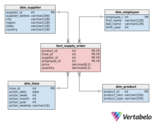
fact_supply_order: contains aggregated data about the order & supplies.
dim_supplier: supplier information.
Advantages
- The fact table is related to each dimension table by exactly one relation.
- Faster aggregations.
- Simpler queries. Relatively fewer joins.
Disadvantages
- Data Integrity is not enforced.
- Data redundancy. City > State > Country can be normalized and not repeated.
Galaxy Schema
Essentially, Galaxy schema can be derived as a collection of star schemas interlinked and completely normalized to avoid redundancy and inaccuracy of data. It is also called Fact Constellation Schema.
Let's combine the above two Star Schemas.
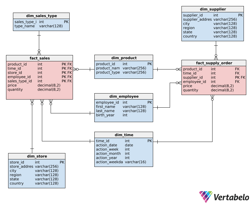
Advantages
- Minimum or no redundancy as a result of Normalization.
- This is a flexible Schema, considering the complexity of the system.
Disadvantages
- Working on this schema is tedious, as Schema and database systems' complexity makes it more intricate.
- Data retrieval is done with multi-level joins combined with conditional expressions.
- The number of levels of normalization is expected, depending on the depth of the given database.
Snowflake Schema
Snowflake is an extension of the Star Schema.
Dimension tables are further normalized and can have their categories.
One or more lookup tables can describe each dimension table. Normalization is recursive until the model is fully normalized.
Check dim_store, dim_product, and dim_time and compare with Star Schema.
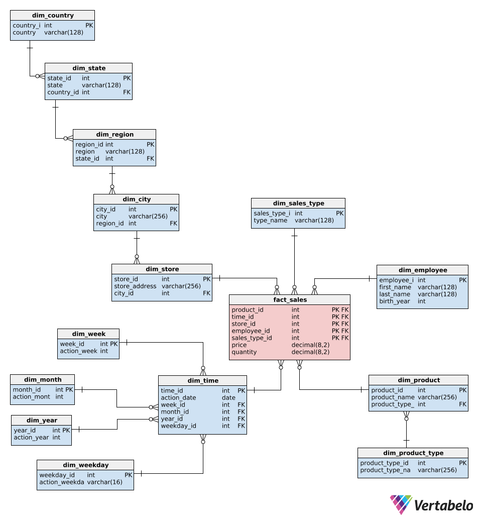
Check the Sales Order Schema
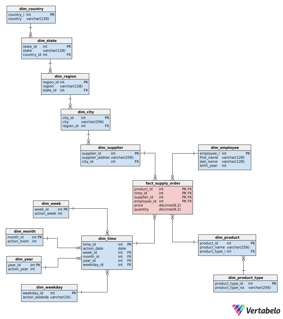
Advantages
Better data quality. Less disk space is used compared to Star Schema.
Disadvantages
The major disadvantage is too many tables to join. Poorly written queries result in a decrease in performance significantly.
Starflake Schema
Starflake = Snow + Snowflake
So how does this work? Some tables are normalized in detail, and some are denormalized.
If used correctly, Starflake schema can give the best of both worlds.
dim_store is normalized, whereas time is denormalized.
Time most of it is int so not much space is wasted and it helps in reducing query complexity.
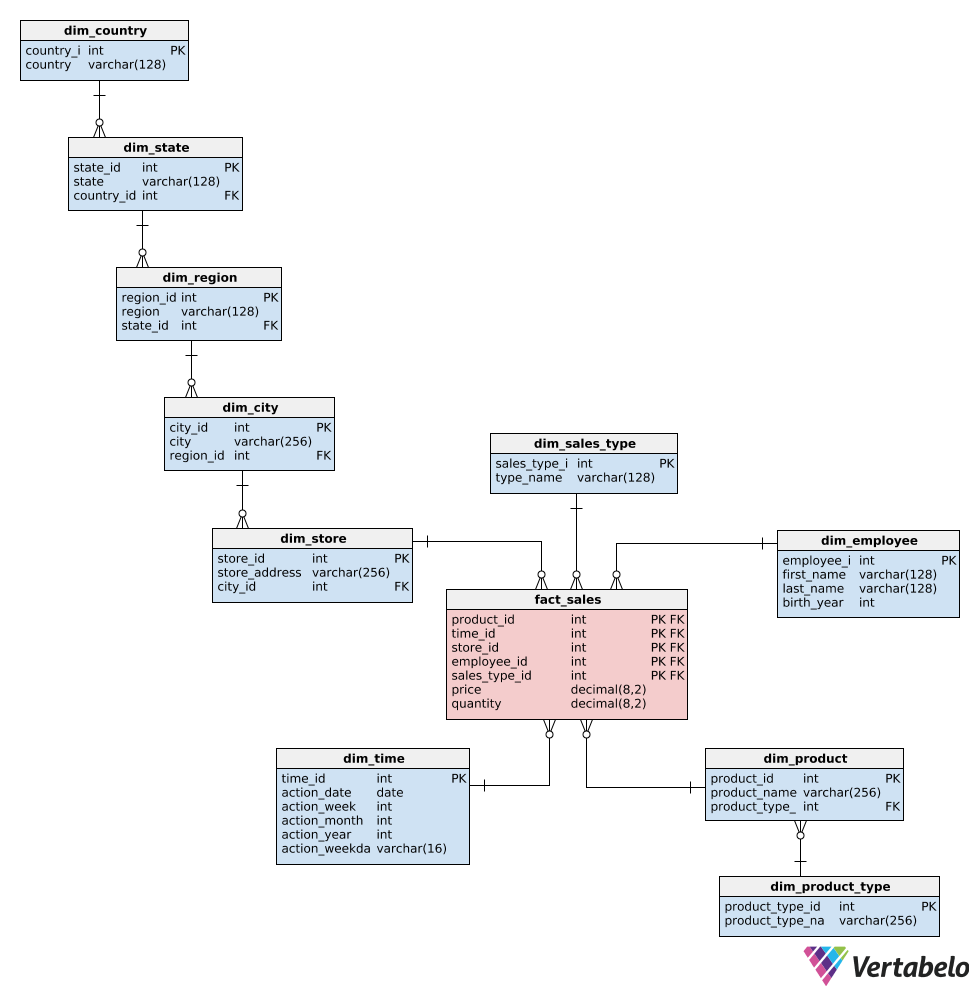
Star vs Snowflake
| Feature | Star Schema | Starflake Schema |
|---|---|---|
| Structure | Single fact table connected to multiple denormalized dimension tables. | Hybrid structure with a mix of denormalized and normalized dimension tables. |
| Complexity | Simple and straightforward, easy to understand and navigate. | More complex due to the normalization of certain dimensions. |
| Data Redundancy | Higher redundancy due to denormalization; data may be duplicated in dimension tables. | Reduced redundancy in normalized parts of the schema, leading to potentially less storage use. |
| Query Performance | Generally faster for query performance because of fewer joins (denormalized data). | Slightly slower query performance due to additional joins needed for normalized tables. |
| Maintenance | Easier to maintain, as there are fewer tables and less complex relationships. | More challenging to maintain, as normalized tables introduce more relationships and dependencies. |
| Flexibility | Less flexible in terms of handling updates and changes in dimension attributes (due to denormalization). | More flexible for handling changes and updates to dimension attributes, as normalization allows for easier updates without affecting the entire table. |
| Use Case | Best for environments where simplicity and query performance are prioritized, such as dashboards and reporting. | Best for environments where data integrity and storage efficiency are critical, and some dimensions require normalization. |
GRAIN
Declaring the grain is the pivotal step in a dimensional design.
The grain establishes precisely what a single fact table row represents.
- Minute-by-minute weather.
- Daily sales.
- A scanner device measures a line item on a customer’s retail sales ticket.
- An individual transaction against an insurance policy.
What is the lowest level data? Grain is defined in business terms, not as rows / columns.
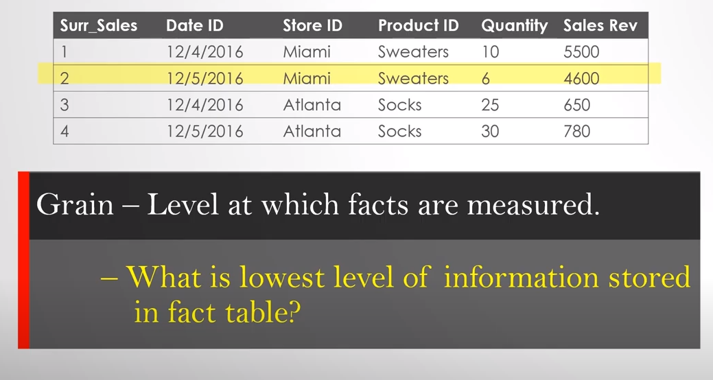
Src: www.aroundbi.com
Based on the image, what do you think as data frequency?
One row per product?
One row per day per product?
One row per day per store per product?
It can be anything, but that has to be decided first.
Ralph Kimball says, "The grain must be declared before choosing dimensions or facts".
The grain must be declared before choosing dimensions or facts because every candidate dimension or fact must be consistent with the grain.
This consistency enforces uniformity on all dimensional designs, that is critical to BI application performance and ease of use.
When changes are made to Grain (adding Per customer to lowest level)
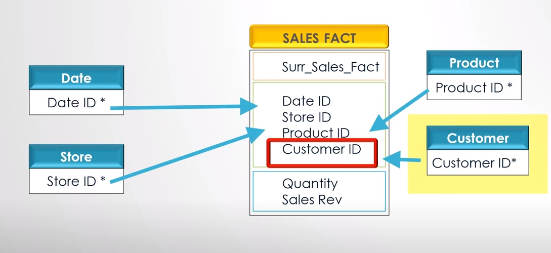
src: www.aroundbi.com
Rolled-up summary grains are essential for performance tuning, but they pre-suppose the business’s common questions.
Each proposed fact table grain results in a separate physical table; different grains must not be mixed in the same fact table.
Making one more change
Helps in Better Reporting. Increases query performance. It helps in getting aggregated / summary view.
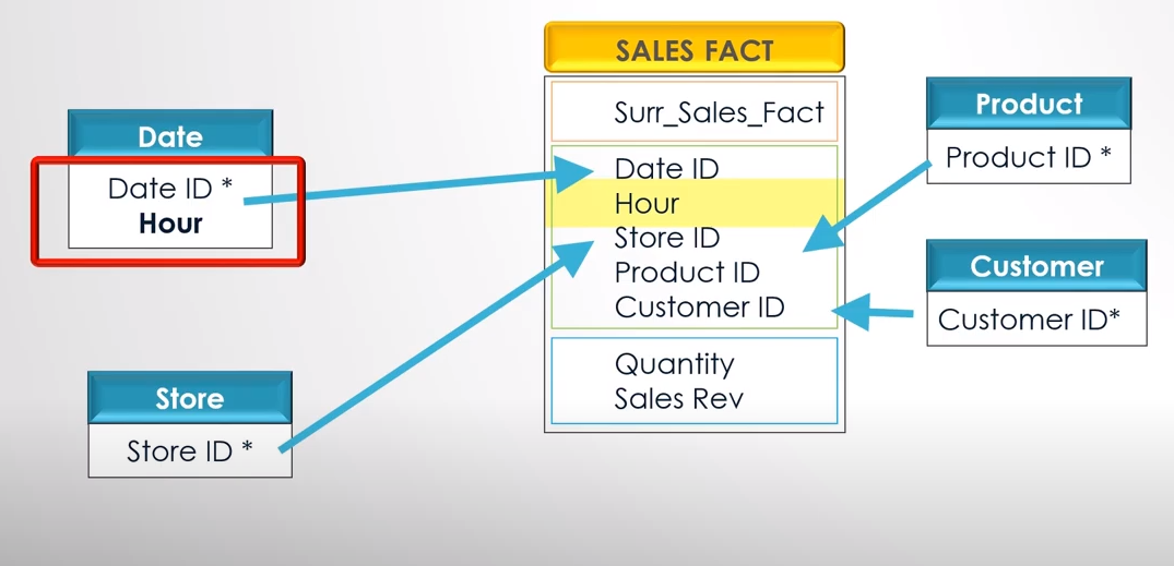
Multi-Fact Star Schema
The schema with more than one fact table linked by normalized dimension tables is often called a "Data Mart Schema" or a "Multi-Fact Star Schema."
This schema can be helpful when you have multiple fact tables that share some but not all dimensions and where the dimensions are normalized.
- Multiple Fact Tables: For different aspects of the business.
- Normalized Dimension Tables: To avoid redundancy and improve data integrity.
It's a complex, real-world adaptation designed to meet specific business needs.
Vertabelo Tool
- Easy to model for any database.
- Model sharing.
- Model exporting.
- Import existing database.
- Easy layout.
- Generate necessary SQL queries.
- Live validation
- SQL Preview.
- Zoom, Navigation, and Search capability.
Dimension - Fact
Identify the Fact and Dimension Tables.
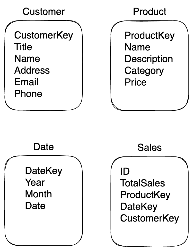
Sample Excercise
From the data given below, Identify the Dimensions and Facts
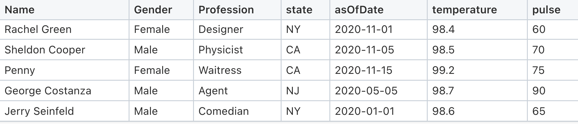
Keys
Again what is Primary Key? Unique - Not Null - One PK per table.
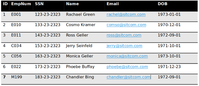
Super Key - A super key is a set or one or more columns (attributes) to identify rows in a table uniquely.
Candidate Key - Minimal super keys with no redundant attributes to uniquely identify a row.
Primary Key - Primary key is selected from the sets of candidate keys.
Alternate Key – A candidate key that was not selected as Primary Key.
Natural Key – A key that happens naturally in the table. Example: SSN, TaxID.
Surrogate Key – A system-generated identifier (Meaningless Simple Number).
Unique Key – Unique values one NULL.
Foreign Key – used to relate other tables.
Super Key
Super Key is a set of one or more columns (attributes) to identify rows in a table uniquely.
For the above table, a bag of keys will help us uniquely identify that table's rows.
{ID}
{EmpNum}
{SSN}
{Email}
{ID,EmpNum}
{ID,SSN}
{ID,Email}
{ID,DOB}
{EmpNum,SSN}
{EmpNum,SSN,Email}
{ID, EmpNum, SSN}
{ID, EmpNum, SSN, DOB}
{ID, EmpNum, SSN, DOB, Name}
{ID, EmpNum, SSN, Name, Email,DOB}
...
Now you get the idea.. we can come up with more & more combinations.
Candidate Key
"Minimal super keys" with no redundant attributes to uniquely identify a row.
Here the essential condition is Minimal. Let's see what minimal keys help us identify a row uniquely.
With just ID, we can uniquely identify a row. Similarly, EmpNum, SSN, and Email can uniquely pull a row.
{ID}

{EmpNum}

{SSN}

{Email}
Primary Key
The primary key is selected from the sets of candidate keys. Let's choose the best column as Primary Key through the process of elimination.
SSN: Sensitive
Email: Varchar
EmpNum: Good to use when needed.
ID: Auto Increment. Widely used in Data Warehousing.
Alternate Key
A candidate key should have been selected as Primary Key.
Email is best suited for Alternate Key. Email can be used to search particular employees if the system doesn’t have access to EmpNum. It is used to link to External accounts.
Surrogate Key
Surrogate Key: A system-generated identifier (Meaningless Simple Number)
ID column matches the definition.
Surrogate Keys are very handy and useful in Data Warehousing.
Unique Key
Unique values may have one NULL value.
Under certain circumstances, Email can be a unique key. Assuming email is generated by a different system and it can be null for a brief period.
Natural Key
A natural key is a column or set of columns that already exist in the table (e.g., they are attributes of the entity within the data model) and uniquely identifies a record in the table. Since these columns are entity attributes, they have business meaning.
Example: SSN
Foreign Key
It is used to refer to other tables.
Why Surrogate Keys are Important
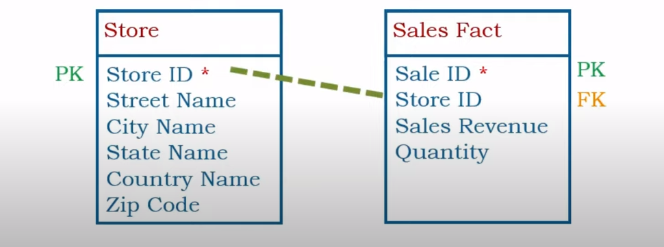
Example of Primary / Foreign Keys
Lets have a sample data
| StoreID * | Street | City | State | Country |
|---|---|---|---|---|
| S1001 | 24th Blvd | Phoenix | AZ | USA |
| S1002 | 21 Bell Road | Miami | FL | USA |
| S1003 | Main Street | New Port | CA | USA |
StoreID is Natural Key (PK) It has a meaning S stands for Store 1001 means its the first store.
What is the issue now ?
When data changes (Slowly Changing Dimension we will cover in next chapter) how to handle the change.
Situation 1: Store 1 moves to new location or store is closed for sometime and opened under new franchise.
| StoreID * | Street | City | State | Country |
|---|---|---|---|---|
| S1001 | 24th Blvd | Phoenix | AZ | USA |
| S1002 | 21 Bell Road | Miami | FL | USA |
| S1003 | Main Street | New Port | CA | USA |
| S1001 | 1st Street | Phoenix | AZ | USA |
Situation 2: When acquiring competitive business (say Target buys KMart), the Natural Keys dont make sense now.
| StoreID * | Street | City | State | Country |
|---|---|---|---|---|
| S1001 | 24th Blvd | Phoenix | AZ | USA |
| S1002 | 21 Bell Road | Miami | FL | USA |
| S1003 | Main Street | New Port | CA | USA |
| 233 | South Street | New Brunswick | NJ | USA |
| 1233 | JFK Blvd | Charlotte | NC | USA |
These business decisions / changes have nothing to do with the Technology.
How to Overcome this issue?
Add Surrogate Keys (running sequence number)
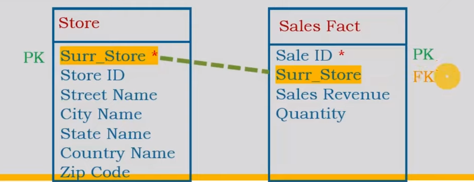
| Surr_Store * | StoreID | Street | City | State | Country |
|---|---|---|---|---|---|
| 1 | S1001 | 24th Blvd | Phoenix | AZ | USA |
| 2 | S1002 | 21 Bell Road | Miami | FL | USA |
| 3 | S1003 | Main Street | New Port | CA | USA |
| 4 | 233 | South Street | New Brunswick | NJ | USA |
| 5 | 1233 | JFK Blvd | Charlotte | NC | USA |
Properties of Surrogate Keys
- Numerical
- Sequential
- Meaningless Simple Number
Adv of Surrogate Keys
- Constant Behavior (will not change based on Business need)
- Integration is easier.
- Faster Query Performance. (because of Integer values)
- Future records (every other column can be NULL still ID is available)
Its a good practice to have Surrogate Key in DataWarehouse Dimension & Fact tables.
More Examples
Dimension columns typically contain descriptive attributes that provide context or categorization to the data, while fact columns contain measurable, numerical data that can be analyzed or aggregated.
Identify the Dimension and Fact in the following designs.
Student Example
| FirstName | LastName | DOB | Ht | Wt | Gender | Course | Grade |
|---|---|---|---|---|---|---|---|
| Ross | Geller | 1967-10-18 | 72 | 170 | Male | Paleontology | A |
| Rachel | Green | 1969-05-05 | 65 | 125 | Female | Fashion Design | B+ |
| Monica | Geller | 1964-04-22 | 66 | 130 | Female | Culinary Arts | A |
| Chandler | Bing | 1968-04-08 | 73 | 180 | Male | Advertising | B |
| Joey | Tribbiani | 1968-01-09 | 71 | 185 | Male | Acting | C+ |
CAR Sales Example
| Manufacturer | Model | Sales_in_thousands | Vehicle_type | Price_in_thousands | Engine_size | Horsepower | Wheelbase | Width | Length | Curb_weight | Fuel_capacity | Fuel_efficiency | Latest_Launch | Power_perf_factor |
|---|---|---|---|---|---|---|---|---|---|---|---|---|---|---|
| Acura | Integra | 16.919 | Passenger | 21.5 | 1.8 | 140 | 101.2 | 67.3 | 172.4 | 2.639 | 13.2 | 28 | 2/2/2012 | 58.28 |
| Acura | TL | 39.384 | Passenger | 28.4 | 3.2 | 225 | 108.1 | 70.3 | 192.9 | 3.517 | 17.2 | 25 | 6/3/2011 | 91.371 |
| Acura | CL | 14.114 | Passenger | [NULL] | 3.2 | 225 | 106.9 | 70.6 | 192 | 3.47 | 17.2 | 26 | 1/4/2012 | [NULL] |
| Acura | RL | 8.588 | Passenger | 42 | 3.5 | 210 | 114.6 | 71.4 | 196.6 | 3.85 | 18 | 22 | 3/10/2011 | 91.39 |
| Audi | A4 | 20.397 | Passenger | 23.99 | 1.8 | 150 | 102.6 | 68.2 | 178 | 2.998 | 16.4 | 27 | 10/8/2011 | 62.778 |
| Audi | A6 | 18.78 | Passenger | 33.95 | 2.8 | 200 | 108.7 | 76.1 | 192 | 3.561 | 18.5 | 22 | 8/9/2011 | 84.565 |
| Audi | A8 | 1.38 | Passenger | 62 | 4.2 | 310 | 113 | 74 | 198.2 | 3.902 | 23.7 | 21 | 2/27/2012 | 134.657 |
| BMW | 323i | 19.747 | Passenger | 26.99 | 2.5 | 170 | 107.3 | 68.4 | 176 | 3.179 | 16.6 | 26 | 6/28/2011 | 71.191 |
Master Data Management
Master Data Management (MDM) refers to creating and managing data that an organization must have as a single master copy, called the master data.
- State
- Customers
- Vendors
- Products
It is the single source of the truth.
MDM is not Data Warehouse but is closely related to Data Warehouse.
Different Goals: MDM is to create and maintain a single source of truth. Whereas in DW, Sales Customer vs. Marketing Customer may differ and not follow a single source of truth.
Types of Data: MDM contains data that doesn't change, mainly Dimensions. At the same time, DW has both Dimensions and Facts.
Reporting Needs: Data Warehousing's priority is to address end-user requirements. MDM's priority is ensuring its follows data governance, quality, and complaint.
Steps of Dimensional Modeling
-
Identify the Business Processes
-
Identify the Facts and Dimensions in your Dimensional Data Model
-
Define the Grain
-
Identify the Attributes / Keys for Dimensions
-
Build the Schema
-
Store Historical Info
Types of Dimensions
- Date Dimension Table
- Degenerate Dimension
- Junk Dimension
- Static Dimension
- Conformed Dimensions
- Slowly Changing Dimensions
- Role Playing Dimension
- Conformed vs Role Playing
- Shrunken Dimension
- Swappable Dimension
- Step Dimension
- Temporal
Date Dimension Table
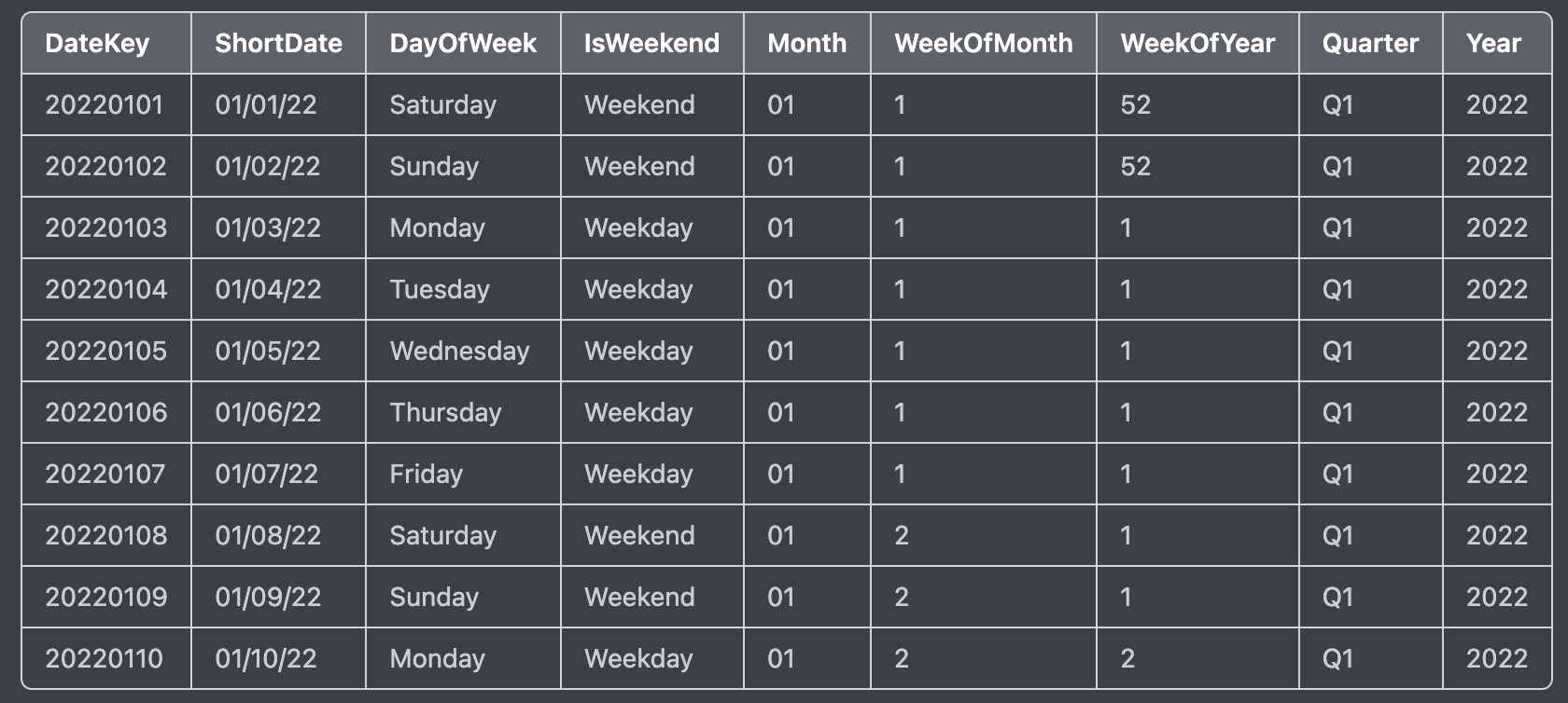
In this example, the Date Dimension table contains information about dates, including the date itself, the year, quarter, month, day, and weekday. The "Date Key" column is the table's primary key and is used to join with other tables in the Star Schema.
This Date Dimension table can be joined with other fact tables in the Star Schema, such as a Sales Fact table, which contains measures such as total sales revenue, units sold, and discounts. By joining the Sales Fact table with the Date Dimension table on the Date Key column, it becomes possible to analyze sales data by date, year, quarter, month, and weekday. For example, it becomes possible to answer questions like:
- What was the total sales revenue for January 2022?
- What were the total units sold on Mondays in Q1 2022?
- What was the average discount percentage on weekends in 2022?
Degenerate Dimension
Generally, what is a Dimension table? Something like a master list. Employee, Product, Date, Store.
In a data warehouse, a degenerate dimension is a dimension key in the fact table that does not have its dimension table.
It is key in the fact table but does not have its dimension table.
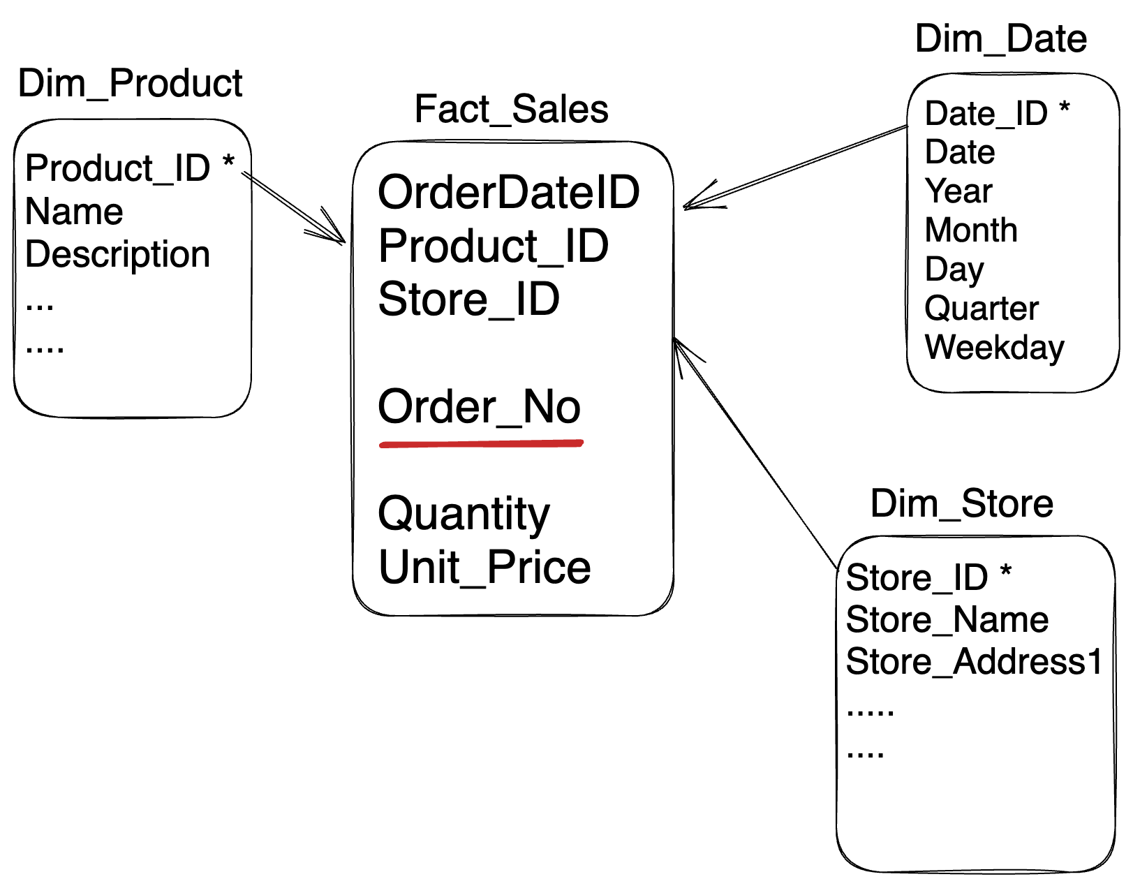
Degenerate dimensions are most familiar with the transaction and accumulating snapshot fact tables.
Means no separate Dimension table.
OrderNo is degenerate dimension. As it has no Dimension table.
Uses of using Degenerate Dimension Table
- Grouping line items
- Getting the average sale
- Tracking
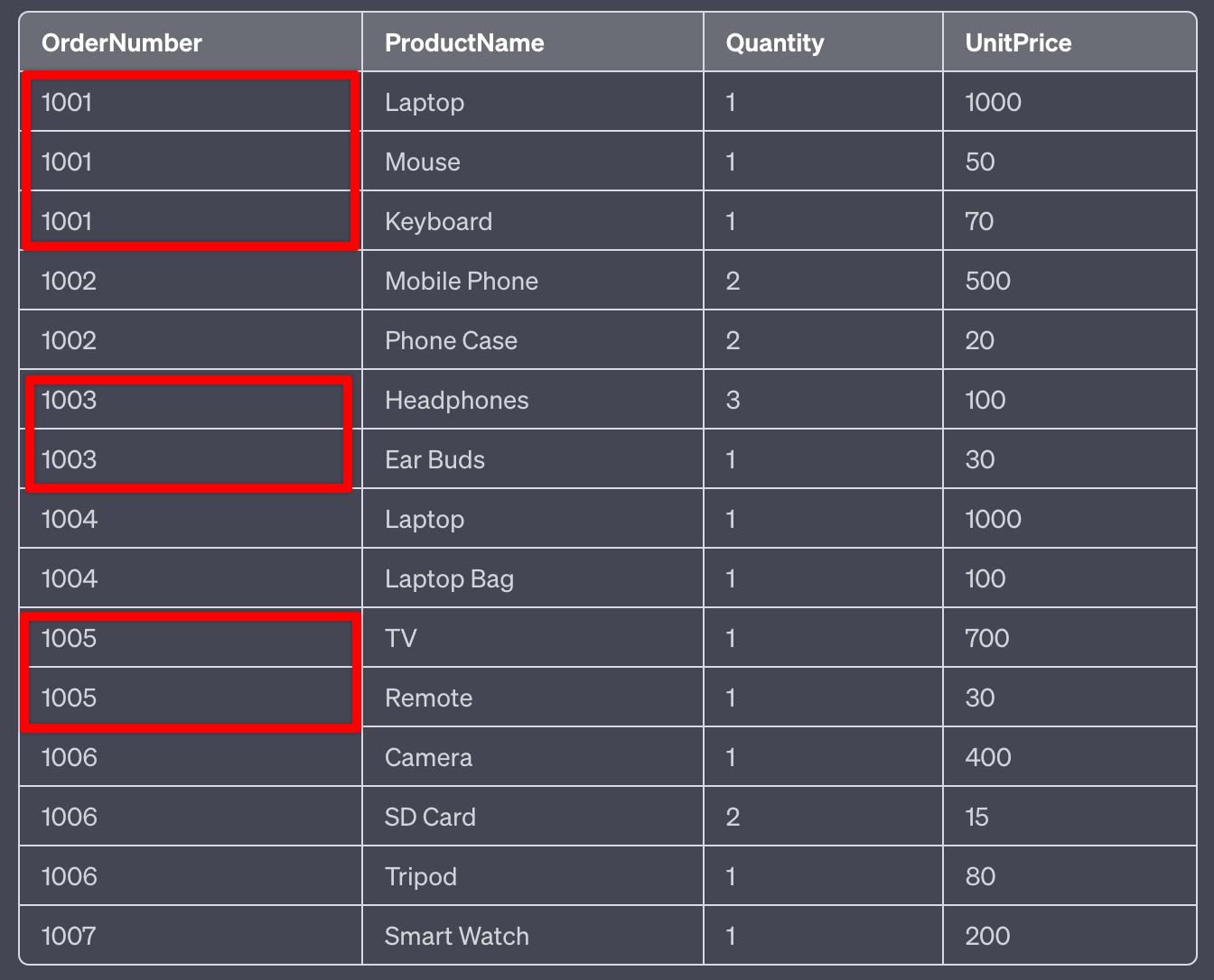
Other Examples of Degenerate Dimensions are
-
Order number or invoice number: This is a typical example of a degenerate dimension. It is a unique identifier for an order or an invoice but has no meaningful attributes other than its value. This degenerate dimension can be used in a fact table to analyze sales by order or invoice number.
-
Tracking number: Another example of a degenerate dimension is a tracking number for a shipment. Like an order number, it is a unique identifier but has no additional attributes associated with it. It can be used in a fact table to analyze shipping performance or delivery times.
-
ATM transaction number: In banking, an ATM transaction number is a unique identifier for a transaction at an ATM. It can be used in a fact table to analyze ATM usage patterns and trends.
-
Serial number: A serial number is a unique identifier assigned to a product or equipment. It can be used in a fact table to analyze the performance of a particular product or equipment.
-
Coupon code: A coupon code is a unique identifier to redeem a discount or promotion. It can be used in a fact table to analyze the usage and effectiveness of different marketing campaigns or promotions.
Degenerate dimensions are helpful when we have a unique identifier for an event or transaction. Still, it has no additional attributes that make it sound like a separate dimension table. In these cases, we can include the unique identifier in the fact table as a degenerate dimension.
Junk Dimension
Cardinality: Number of Unique Values.
A junk dimension is a dimension table created by grouping low cardinality and unrelated attributes.
The idea behind a junk dimension is to reduce the number of dimension tables in a data warehouse and simplify queries.
An example of a junk dimension could be a table that includes binary flags such as "is_promotion", "is_return", and "is_discount".
Possible Values for is_promotion as Y or N same for is_return and is_discount.
Example:
fact_sale table
Date
Product
Store
OrderNumber

PaymentMode
StoreType
CustomerSupport

Quantity
UnitPrice
Possible values for these columns
PaymentMode - Cash/Credit/Check
StoreType - Warehouse/Marketplace
CustomerSupport - Yes/No
So how to handle the situation
Option 1: Add it to Fact Table

The problem is, Fact table data is not that important and sometimes won't make sense
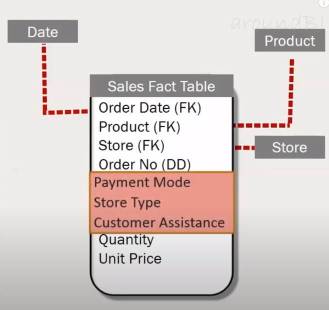
src: aroundbi.com
Option 2: Add it as Dimension Table

The problem is with more Dimension table adds more joins to your queries.
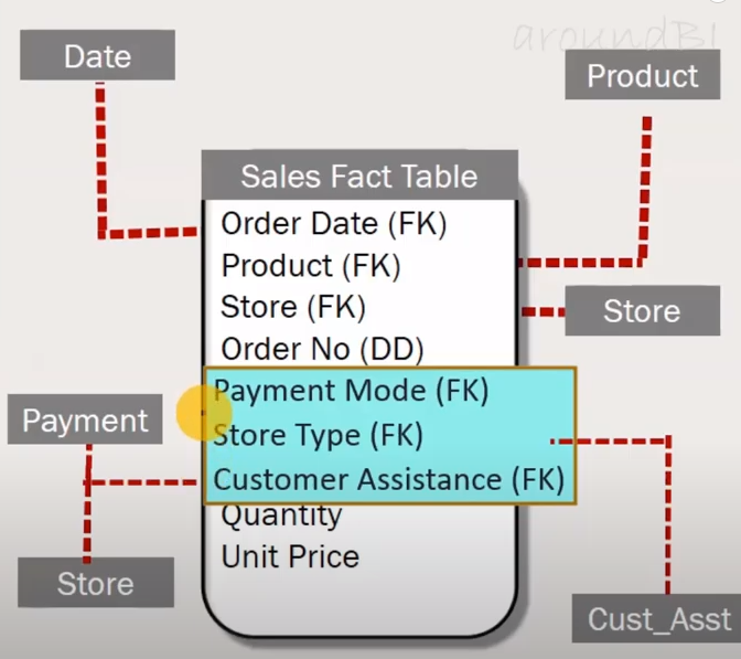
src: aroundbi.com
Do you know how to take care of this situation?
Let's create a new table with values from all possible combinations.
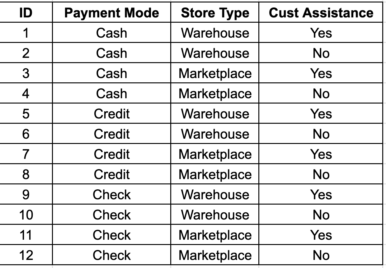
Junk Dimension with ID
So, the revised Fact Table looks like this
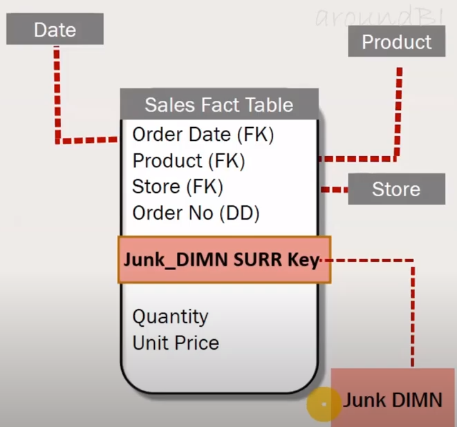
- Basically to group low cardinality columns.
- If the values are too uncorrelated.
- Helps to keep the DW simple by minimizing the dimensions.
- Helps to improve the performance of SQL queries.
Note: If the resultant dimension has way too many rows, then don’t create a Junk dimension.
Static Dimension
A static dimension refers to a dimension table in a data warehouse that does not change or infrequently changes over time.
Values Never Change.
Time Dimension: Days, weeks, months
Payment Method Dimension: Credit Card, Debit Card, PayPal, Zelle, etc.
Education Level Dimension: High School, Bachelor, Master, PhD, etc.
Geographic Dimension: Store Locations, Categories, US States, Countries, etc.
Conformed Dimensions
This dimension is consistent and the same across multiple fact tables in a data warehouse. The dimension tables are designed once and used across various areas, maintaining consistency.
List of countries/states where the company is doing business.
An excellent example of a conformed dimension is a "Date" or "Time" dimension. Imagine a data warehouse for a retail business that has two fact tables: "Sales" and "Inventory". These fact tables might have a "Date" dimension that tracks when a sale or inventory count was made.
In this example, Date, Product, and Store dimensions remain constant across multiple fact tables.
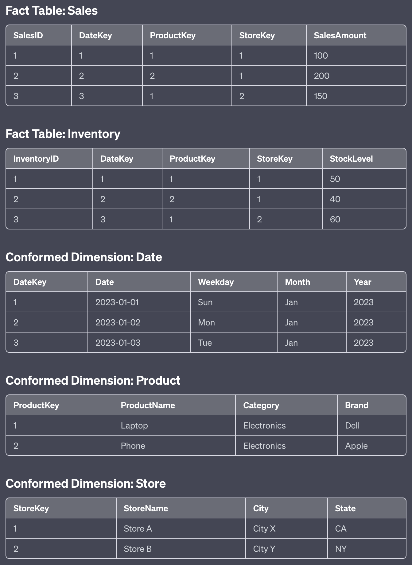
Slowly Changing Dimensions
Slowly Changing Dimensions (SCDs) is a concept in data warehousing and business intelligence that deals with managing changes in dimension data over time.
Data Warehousing has

- Time Variant (with history data)
- Non Volatile (no changes)

But in reality

- The customer may change his address.
- Store move to a new location.
- An employee joins a new company.
Dimension data refers to the descriptive attributes of an entity, such as customer, product, or location. These attributes provide context for analysis and reporting in a data warehouse.
However, dimension data can change over time, and it's essential to maintain a historical record of these changes for accurate reporting and analysis.
There are several types of SCDs, each with different strategies for managing changes in dimension data:
Type 1 - Overwrite: In this approach, when changes occur, the existing values are overwritten with the new values. No historical data is preserved.
Type 2 - Add a New Row: This method maintains a complete history of changes by adding a new row with the updated attribute values in the dimension table. Each row has a start and end date (or a start date and a flag indicating the current record) to show the period during which the attribute values were valid.
Type 3 - Add a New Column: This approach maintains a limited history of changes by adding new columns to the dimension table to store the previous values of changed attributes. It is useful when tracking a small number of changes but can become unwieldy with many changes.
Type 4 - Add a History Table: In this method, a separate history table stores the changes in the dimension attributes. The primary dimension table contains the current attribute values, while the history table stores historical data.
Type 6 - Hybrid: This combines Type 1, Type 2, and Type 3 approaches. It allows for the selective preservation of history for specific attributes and can be used to overwrite certain attribute values.
Choosing the appropriate SCD type depends on the specific requirements of the data warehouse, the importance of historical data for analysis, and the performance implications of each approach.
SCD - Type 0
Type 0 - Retain Original: This approach ignores changes and retains the original values for the dimension attributes. No history is kept for changes.
The Product dimension table might include the following columns:
- Product_ID
- Product_Name
- Category
- Price
Now, imagine that the store decides to re-categorize one of its products. For instance, they may change the "Smartphone" product from the "Electronics" category to the "Mobile Devices" category.
Using a Type 0 Slowly Changing Dimension approach, the store will retain the original value for the product category, ignoring the change. In this case, the Product dimension table would still show the "Smartphone" product in the "Electronics" category, even though it has been re-categorized to "Mobile Devices." This approach means no history is kept for changes, and the original values are always preserved.
The Product dimension table would look like this:
| Product_ID | Product_Name | Category | Price |
|---|---|---|---|
| 1 | Smartphone | Electronics | 1000 |
Use Cases:
- When historical data is not relevant or necessary for analysis, and only the original values are needed.
- For dimensions with attributes that are fixed and don't change over time, such as unique identifiers or codes.
- In cases where the data warehouse is only required to support reporting and analysis on the current state of the business and not the historical trends.
Advantages:
- Simplicity: SCD Type 0 is the simplest approach, as it doesn't require any additional mechanisms to handle changes in dimension attributes.
- Space Efficiency: Since there is no need to store historical data or multiple versions of records, the dimension tables will be smaller and require less storage space.
- Performance: As there are no additional rows or columns for historical data, the querying and processing of the data warehouse will generally be faster.
Disadvantages:
- Lack of Historical Data: SCD Type 0 does not store any historical data, which means it cannot support reporting and analysis that requires tracking changes over time. This can be a significant limitation for businesses that need to analyze trends, understand the impact of changes, or perform other historical analyses.
- Inaccurate Analysis: Since the dimension table only contains the original values, any changes that have occurred over time are not reflected. This may lead to incorrect analysis results or conclusions based on outdated information.
- Inability to Track Changes: With SCD Type 0, it is impossible to determine when or why changes occurred, as there is no record of any changes in the dimension data.
SCD - Type 1
Type 1 - Overwrite: In this approach, when changes occur, the existing values are overwritten with the new values. No historical data is preserved.
Before the change, the Product dimension table looks like this:
| Product_ID | Product_Name | Category | Price |
|---|---|---|---|
| 1 | Smartphone | Electronics | 800 |
After the change, the Product dimension table will look like this:
| Product_ID | Product_Name | Category | Price |
|---|---|---|---|
| 1 | Smartphone | Mobile Devices | 800 |
With a Type 1 SCD approach, the table now reflects the updated category for the "Smartphone" product. However, there is no record of the product's previous category, "Electronics," in the table.
Use Cases:
- When historical data is not essential for analysis, and only the current values are needed.
- For dimensions where tracking historical changes is not required for the business, such as minor corrections or updates to attributes.
- In cases where the data warehouse is required to support reporting and analysis on the current state of the business, and not historical trends.
Advantages:
- Simplicity: SCD Type 1 is relatively simple to implement, as it only requires overwriting existing records when changes occur.
- Space Efficiency: Since there is no need to store historical data or multiple versions of records, the dimension tables will be smaller and require less storage space.
- Performance: As there are no additional rows or columns for historical data, the querying and processing of the data warehouse will generally be faster.
Disadvantages:
- Lack of Historical Data: SCD Type 1 does not store any historical data, which means it cannot support reporting and analysis that requires tracking changes over time. This can be a significant limitation for businesses that need to analyze trends, understand the impact of changes, or perform other historical analyses.
- Loss of Previous Data: Since the dimension table only contains the most recent values, any changes that have occurred over time overwrite the previous values. This may lead to a loss of potentially valuable historical information.
- Inability to Track Changes: With SCD Type 1, it is impossible to determine when or why changes occurred, as there is no record of any changes in the dimension data. This can make it challenging to understand the reasons for changes or identify any potential issues or patterns.
SCD - Type 2
Using the retail store example with the "Product" dimension, let's see how a Type 2 Slowly Changing Dimension approach would handle the change in the product category.
Recall that the Product dimension table contains the following columns:
- Product_ID
- Product_Name
- Category
- Price
For a Type 2 SCD, we will need to add two additional columns to the table:
- Start_Date
- End_Date (or a flag indicating the current record, such as "Is_Current")
Now, imagine that the store decides to re-categorize the "Smartphone" product from the "Electronics" category to the "Mobile Devices" category, as in the previous examples.
With a Type 2 SCD approach, the store will add a new row with the updated category information while retaining the old row in the table. Each row will have a start and end date, indicating the period during which the attribute values were valid.
Before the change, the Product dimension table looks like this:
| Product_ID | Product_Name | Category | Price | Start_Date | End_Date |
|---|---|---|---|---|---|
| 1 | Smartphone | Electronics | 800 | 2021-01-01 | NULL |
After the change, the Product dimension table will look like this:
| Sur_ID | Product_ID | Product_Name | Category | Price | Start_Date | End_Date |
|---|---|---|---|---|---|---|
| 1 | 1 | Smartphone | Electronics | 800 | 2021-01-01 | 2023-04-03 |
| 2 | 1 | Smartphone | Mobile Devices | 800 | 2023-04-04 | NULL |
With a Type 2 SCD approach, the table now has a new row reflecting the updated category for the "Smartphone" product.
Additionally, the previous row for the "Smartphone" product with the "Electronics" category is still in the table, with an updated End_Date.
This approach allows for the preservation of historical data and enables accurate reporting and analysis based on the product's category at different points in time.
Use Cases:
- When historical data is critical for analysis, and it's essential to track changes over time for reporting and decision-making.
- For dimensions where understanding the impact of changes on business performance, such as customer demographics, product attributes, or pricing, is vital.
- In cases where the data warehouse is required to support reporting and analysis that includes historical trends, comparisons, and the effect of changes over time.
Advantages:
- Historical Data Preservation: SCD Type 2 maintains a complete history of changes in the dimension attributes, enabling more accurate and detailed reporting and analysis.
- Accurate Analysis: By preserving historical data, SCD Type 2 allows for accurate analysis and reporting that accounts for changes over time, leading to better insights and decision-making.
- Change Tracking: SCD Type 2 enables tracking of when and why changes occurred, making it easier to identify patterns, trends, or potential issues in the dimension data.
Disadvantages:
- Complexity: SCD Type 2 is more complex to implement and manage compared to SCD Type 0 and Type 1, as it requires additional mechanisms to handle changes in dimension attributes and maintain historical data.
- Space Requirements: Since multiple versions of records are stored to maintain historical data, the dimension tables will be larger and require more storage space.
- Performance: As there are additional rows for historical data, the querying and processing of the data warehouse may be slower compared to SCD Type 0 or Type 1, especially when dealing with large amounts of historical data. This may require more robust indexing, partitioning, or query optimization strategies to maintain acceptable performance.
SCD - Type 3
SCD Type 3 involves adding a new column to the dimension table to store the previous value of the changed attribute along with the current value. It allows tracking the current and previous values but needs to maintain a complete history of changes. Using the same "Product" dimension example with the mobile product category change:
Recall that the Product dimension table contains the following columns:
- Product_ID
- Product_Name
- Category
- Price
For a Type 3 SCD, we will need to add a column to the table:
- Previous_Category
Now, imagine that the store decides to re-categorize the "Smartphone" product from the "Electronics" category to the "Mobile Devices" category, as in the previous examples.
With a Type 3 SCD approach, the store will update the existing row by setting the "Previous_Category" column to the old category value and overwriting the "Category" column with the new value.
Before the change, the Product dimension table looks like this:
| Product_ID | Product_Name | Category | Price | Previous_Category |
|---|---|---|---|---|
| 1 | Smartphone | Electronics | 800 | NULL |
After the change, the Product dimension table will look like this:
| Product_ID | Product_Name | Category | Price | Previous_Category |
|---|---|---|---|---|
| 1 | Smartphone | Mobile Devices | 800 | Electronics |
With a Type 3 SCD approach, the table now reflects the updated category for the "Smartphone" product and also retains the previous category in the "Previous_Category" column. However, it can only track one previous value and does not maintain a complete history of all changes that occurred over time.
Use Cases:
-
When it is essential to track the immediate previous value of an attribute, but a complete history of changes is not required.
-
For dimensions where the primary focus is on comparing the current value with the previous value, rather than analyzing historical trends.
-
In cases where the data warehouse is required to support reporting and analysis that involves comparisons between current and previous states, but not a full history of changes.
Advantages:
-
Limited Historical Data: SCD Type 3 preserves the immediate previous value of an attribute, allowing for some level of historical analysis and comparison with the current value.
-
Space Efficiency: Since only one previous value is stored, the dimension tables will require less storage space compared to SCD Type 2.
-
Simplicity: SCD Type 3 is relatively simple to implement, as it only requires adding a new column to the dimension table and updating it when changes occur.
Disadvantages:
-
Incomplete Historical Data: SCD Type 3 does not maintain a full history of changes, which may limit the depth of historical analysis and reporting that can be performed.
-
Limited Change Tracking: With SCD Type 3, it is only possible to track the immediate previous value of an attribute, making it difficult to understand trends or patterns in the data over time.
-
Additional Columns: SCD Type 3 requires adding a new column for each attribute that needs to track the previous value, which can increase the complexity of the dimension table schema.
-
Scalability: If there are multiple attributes that require tracking of previous values or if the number of changes becomes more frequent, SCD Type 3 may become less practical and harder to manage. In such cases, SCD Type 2 may be a more suitable approach to maintain a complete history of changes.
Suppose the university decides to change the credit hours of a specific course, "Introduction to Data Science," from 3 to 4 credit hours. The university wants to track both the current and the immediately previous credit hours for reporting purposes.
Using SCD Type 3, the university would update the course's record in the Course dimension table by overwriting the "Credit_Hours" column and updating the "Previous_Credit_Hours" column with the old value.
Before the change, the Course dimension table looks like this:
| Course_ID | Course_Name | Credit_Hours | Previous_Credit_Hours |
|---|---|---|---|
| 1 | Introduction to Data Science | 3 | NULL |
After the change, the Course dimension table will look like this:
| Course_ID | Course_Name | Credit_Hours | Previous_Credit_Hours |
|---|---|---|---|
| 1 | Introduction to Data Science | 4 | 3 |
With a Type 3 SCD approach, the table now reflects the updated credit hours for the "Introduction to Data Science" course and retains the previous credit hours in the "Previous_Credit_Hours" column. This allows the university to compare the current and previous credit hours, which might be useful for understanding recent changes in course workload. However, it does not maintain a complete history of all credit hour changes over time.
SCD - Type 4
SCD Type 4, the "history table" approach, involves creating a separate table to store historical data, while the main dimension table only retains current information. Using the "Product" dimension example with the mobile product category change:
Recall that the Product dimension table contains the following columns:
- Product_ID
- Product_Name
- Category
- Price
For a Type 4 SCD, we will create an additional table called "Product_History":
Product_History Table:
- History_ID
- Product_ID
- Category
- Price
- Valid_From
- Valid_To
Now, imagine that the store decides to re-categorize the "Smartphone" product from the "Electronics" category to the "Mobile Devices" category.
With a Type 4 SCD approach, the store will insert a new row in the "Product_History" table, representing the previous state of the "Smartphone" product, and update the existing row in the main "Product" dimension table with the new category.
Before the change, the tables look like this:
Product Dimension Table:
| Product_ID | Product_Name | Category | Price |
|---|---|---|---|
| 1 | Smartphone | Electronics | 800 |
Product_History Table:
(empty)
After the change, the tables will look like this:
Product Dimension Table:
| Product_ID | Product_Name | Category | Price |
|---|---|---|---|
| 1 | Smartphone | Mobile Devices | 800 |
Product_History Table:
| History_ID | Product_ID | Category | Price | Valid_From | Valid_To |
|---|---|---|---|---|---|
| 1 | 1 | Electronics | 800 | 2020-01-01 | 2023-01-01 |
With a Type 4 SCD approach, the main "Product" dimension table contains only the current information, and the "Product_History" table maintains the history of changes. This approach helps maintain a clean dimension table and allows for efficient querying of current data while still preserving historical data for analysis when required.
Use Cases:
-
When it is important to maintain a complete history of changes, but the main dimension table should only contain the current state of the data.
-
For situations where querying the current data efficiently is a priority, but historical data is still required for more in-depth analysis.
-
When the dimension table is frequently accessed or queried for current data, and performance is a concern.
Advantages:
-
Performance: By keeping the current data in the main dimension table and historical data in a separate table, SCD Type 4 allows for efficient querying of the current data without the overhead of historical data.
-
Historical Data: SCD Type 4 maintains a complete history of changes, enabling in-depth analysis and reporting that requires historical data.
-
Separation of Concerns: By separating the current and historical data, SCD Type 4 provides a cleaner and more organized data structure, making it easier to manage and maintain.
-
Scalability: Since historical data is stored separately, SCD Type 4 can scale well with large dimensions and frequent changes.
Disadvantages:
-
Complexity: SCD Type 4 adds complexity to the data warehouse design and maintenance, as it requires managing two separate tables for the same dimension.
-
Increased Storage: Storing historical data in a separate table requires additional storage space, which can be a concern for large dimensions with extensive change history.
-
Maintenance: Implementing and maintaining SCD Type 4 can be more challenging than other SCD types, as it requires managing the relationships between the dimension and history tables and ensuring data integrity between them.
-
Query Complexity: Analyzing historical data and comparing it with current data can involve more complex queries, as it may require joining the dimension and history tables.
Overall, SCD Type 4 is suitable for scenarios where maintaining a complete history of changes is necessary, but the main dimension table should only contain the current state of the data to optimize query performance.
SCD - Type 6
SCD Type 6 is a hybrid approach that combines the features of SCD Types 1, 2, and 3. It maintains the current attribute value, the previous attribute value, and a full history of changes with effective dates. Using the "Product" dimension example with the mobile product category change:
Recall that the Product dimension table contains the following columns:
- Product_ID
- Product_Name
- Category
- Price
For a Type 6 SCD, we will need to add the following columns to the table:
- Previous_Category
- Valid_From
- Valid_To
- Is_Current
Now, imagine that the store decides to re-categorize the "Smartphone" product from the "Electronics" category to the "Mobile Devices" category.
With a Type 6 SCD approach, the store will insert a new row in the "Product" dimension table with the updated category and set "Is_Current" to 'Y' (Yes) for the new row and 'N' (No) for the old row. The new row will have the "Previous_Category" column set to the old category value.
Before the change, the Product dimension table looks like this:
| Product_ID | Product_Name | Category | Price | Previous_Category | Valid_From | Valid_To | Is_Current |
|---|---|---|---|---|---|---|---|
| 1 | Smartphone | Electronics | 800 | NULL | 2020-01-01 | NULL | Y |
After the change, the Product dimension table will look like this:
| Product_ID | Product_Name | Category | Price | Previous_Category | Valid_From | Valid_To | Is_Current |
|---|---|---|---|---|---|---|---|
| 1 | Smartphone | Electronics | 800 | NULL | 2020-01-01 | 2023-01-01 | N |
| 2 | Smartphone | Mobile Devices | 800 | Electronics | 2023-01-01 | NULL | Y |
With a Type 6 SCD approach, the table now reflects the updated category for the "Smartphone" product, retains the previous category, and maintains a full history of changes with effective dates. This approach provides the benefits of SCD Types 1, 2, and 3 while optimizing the storage and query performance to some extent. However, it still requires managing additional columns and more complex logic for managing the Is_Current flag and Valid_From/Valid_To dates.
SCD - Type 5 - Fun Fact
A data warehousing expert, Ralph Kimball, introduced the concept of Slowly Changing Dimensions and defined Types 0, 1, 2, and 3. These widely adopted types became the standard classification for handling dimension changes.
Later, other types, such as Type 4 and Type 6, were proposed by different practitioners to address additional scenarios and use cases that needed to be covered by Kimball's original classification. However, there was no commonly agreed upon and widely adopted SCD Type 5.
In short, SCD Type 5 does not exist because it was never proposed or documented as a distinct method for handling dimension changes. The existing SCD types (0, 1, 2, 3, 4, and 6) cover most use cases and have been widely adopted in the data warehousing community.
Role Playing Dimension
Role-playing dimension is a term used in data warehousing that refers to a dimension used for multiple purposes within the same database. Essentially, the same dimension table is linked to the fact table multiple times, each playing a different role. This concept is often used when a single physical dimension can have different meanings in other contexts.
Date Dimension: This is the most common example. A single date dimension table can be used to represent different types of dates in a fact table, such as:
- Order Date: The date when an order was placed.
- Shipping Date: The date when an order was shipped.
- Delivery Date: The date when an order was delivered.
Employee Dimension in a Hospital Setting:
- Attending Physician: The primary doctor responsible for a patient.
- Referring Physician: The doctor who referred the patient to the hospital.
- Admitting Physician: The doctor who admitted the patient to the hospital.
Product Dimension in Retail:
- Ordered Product: The product that a customer ordered.
- Returned Product: The product that a customer returned.
- Replacement Product: The product was sent as a replacement for a returned item.
Why Use Role-Playing Dimensions?
- Efficiency: It's efficient in terms of storage as you don't need to create multiple dimension tables for each role.
- Consistency: Ensures consistency across different business processes since the same dimension table is used.
- Flexibility: Offers flexibility in querying and reporting. You can easily compare and contrast different aspects (like order date vs. delivery date).
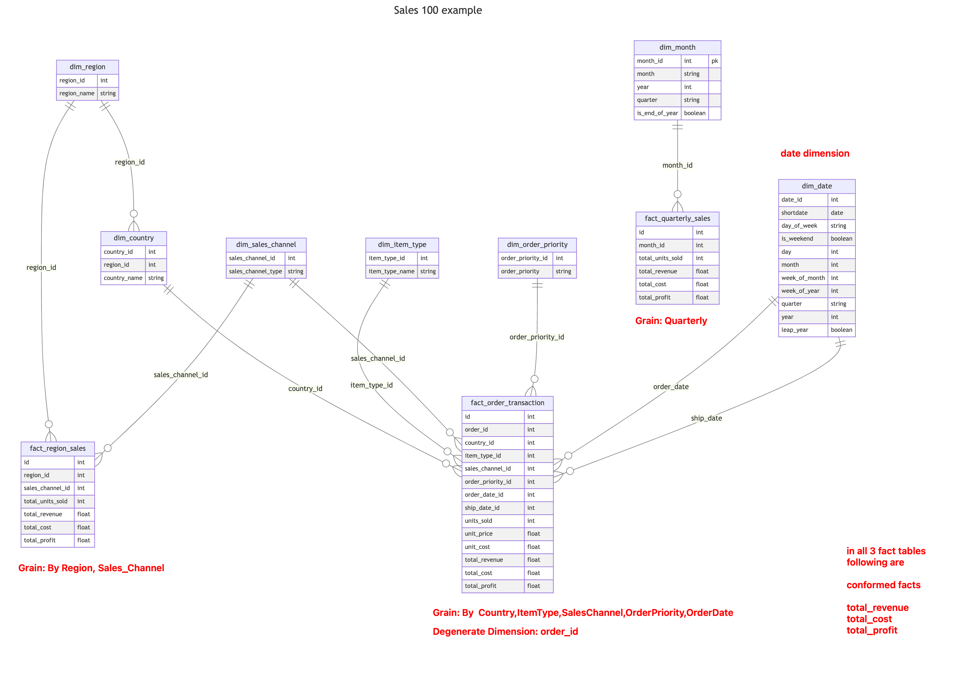
Conformed vs Role Playing
Conformed and role-playing dimensions are both concepts in data warehousing, but they serve different purposes.
A conformed dimension is a dimension that is shared across multiple fact tables in a data warehouse. A conformed dimension has the same meaning and structure in all fact tables and is used to maintain consistency and integrity in the data warehouse.
For example, a Date dimension could be used in multiple fact tables that record sales, inventory, and customer data. The Date dimension maintains its structure and meaning across all fact tables, ensuring consistent and accurate analysis.
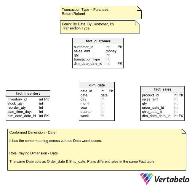
Shrunken Dimension
A shrunken dimension is a subset of a dimension’s attributes that apply to a higher summary level. For example, a Month dimension would be a shrunken dimension of the Date dimension. The Month dimension could be connected to a forecast fact table whose grain is at the monthly level.
(Sales Dimension Example)
Suppose you have a dataset with 100 features (or variables) that describe some phenomenon. However, you suspect that not all of these features are relevant to predicting the outcome you're interested in. You suspect many of these features are noisy, redundant, or irrelevant.
CREATE TABLE dim_patient (
    PatientID INT PRIMARY KEY,
    Name STRING,
    Age INT,
    Gender STRING,
    Race STRING,
    Height DECIMAL,
    Weight DECIMAL,
    EyeColor STRING,
    MaritalStatus STRING,
    Address STRING,
    City STRING,
    State STRING,
    ZipCode STRING,
    PhoneNumber STRING,
    EmailAddress STRING,
    InsuranceProvider STRING,
    InsurancePolicyNumber STRING,
    PrimaryCarePhysician STRING
);
In this shrunken dimension, you're reducing the attribute set to only those necessary for BMI analysis, simplifying the data model for this specific use case.
CREATE TABLE dim_patient_bmi(
    PatientID INT Primary KEY,
    Name String,
    Height DECIMAL,
    Weight DECIMAL,
    BMI DECIMAL
)


CREATE TABLE dim_patient_demographics (
    PatientID INT PRIMARY KEY,
    Age INT,
    Gender STRING,
    Race STRING
);
Swappable Dimension
Swappable dimensions are used in data warehousing when you have multiple versions of a dimension and you want to switch between them for different types of analysis. This concept is particularly useful in scenarios where different perspectives or classifications are needed for the same underlying data.
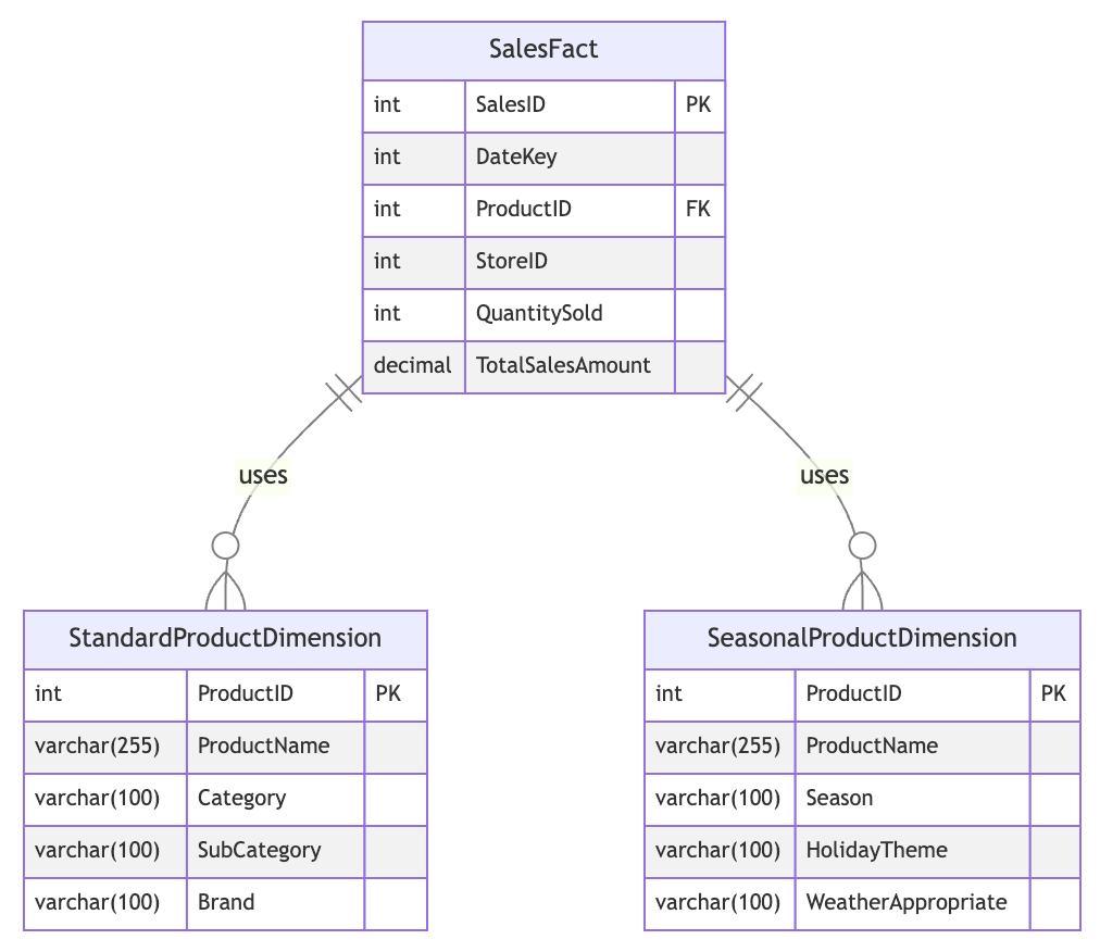
Key Components
Fact Table: SalesFact
Contains measures like QuantitySold and TotalSalesAmount Has a foreign key (ProductID) that can link to either product dimension
Multiple Dimension Tables:
- StandardProductDimension
- SeasonalProductDimension
Common Identifier:
Both dimension tables share ProductID as their primary key
Different Attributes:
- StandardProductDimension: Category, SubCategory, Brand
- SeasonalProductDimension: Season, HolidayTheme, WeatherAppropriate
Functionality:
Allows switching between different product perspectives in analyses Enables querying sales data using either standard or seasonal product attributes
Benefits:
- Flexibility in reporting and analysis
- Accommodates different business needs or seasonality
- Optimizes storage by separating rarely-used attributes
Use Case Example:
- Use StandardProductDimension for regular inventory analysis
- Switch to SeasonalProductDimension for holiday sales planning
Implementation Note: Requires careful ETL processes to ensure data consistency across dimensions.
Step Dimension
A Step Dimension in data warehousing represents a process that involves several steps or stages, each of which might need to be analyzed separately. This type of dimension is beneficial in scenarios where a process progresses through distinct phases, and you want to track or analyze each phase individually.
Step Dimension: OrderStatusDimension
This dimension table represents the different steps in the order processing lifecycle.
CREATE TABLE OrderStatusDimension (
    StatusID INT PRIMARY KEY,
    StatusName VARCHAR(100),
    Description VARCHAR(255)
);
| StatusID | StatusName | Description |
|---|---|---|
| 1 | Order Placed | Order has been placed |
| 2 | Payment Processed | Payment has been received |
| 3 | Shipped | Order has been shipped |
| 4 | Delivered | Order has been delivered |
Fact Table: OrderFact
The fact table tracks each order along with its current status.
CREATE TABLE OrderFact (
    OrderID INT PRIMARY KEY,
    DateKey INT,
    CustomerID INT,
    ProductID INT,
    StatusID INT,  -- Foreign Key to OrderStatusDimension
    Quantity INT,
    TotalAmount DECIMAL
);
SQL Query Example
To analyze the number of orders at each status:
SELECT
    osd.StatusName,
    COUNT(*) AS NumberOfOrders
FROM
    OrderFact of
JOIN
    OrderStatusDimension osd ON of.StatusID = osd.StatusID
GROUP BY
    osd.StatusName;
Remember the Accumulating Snapshot Fact table?
Step dimensions are closely connected to the Accumulating Snapshot Fact table.
CREATE TABLE OrderProcessFact (
    OrderID INT PRIMARY KEY,
    CustomerID INT,
    ProductID INT,
    OrderDate DATE,
    PaymentDate DATE NULL,
    ShipDate DATE NULL,
    DeliveryDate DATE NULL,
    QuantityOrdered INT,
    TotalAmount DECIMAL,
    CurrentStatus VARCHAR(100)
);
- When an order is placed, a new record is inserted with the
OrderDateand initialCurrentStatus. - As the order progresses through payment, shipping, and delivery, the respective date fields and the
CurrentStatusare updated. - This table allows for analysis of the duration between different stages of the order process, identification of bottlenecks, and overall process efficiency.
Temporal
Temporal refers to anything related to time. In the context of databases, data warehousing, and analytics, "temporal" generally describes aspects that change or evolve over time, or that are connected to the tracking of time.
Examples
Temporal Data: Data that represents a point or duration in time. This can include:
- Timestamps: A specific point in time (e.g., "2020-10-15 10:30:00").
- Dates: A particular day, month, or year (e.g., "2020-10-15").
- Time Ranges: A start and end date (e.g., "2020-10-01 to 2020-10-15").
Temporal Dimension: A dimension (like dim_date or dim_time) that stores and manages information about time. It's used in queries to analyze data based on time intervals (e.g., sales per month, inventory levels over time).
Temporal Relationships: These are relationships between entities that change over time. For example, in customer data, an individual might change their address, and you may want to track how that address evolves over time.
Temporal Analysis: Analyzing how things change over time, such as:
- Trend Analysis: How sales grow or decline over time.
- Duration Analysis: How long an order stays in each processing step.
- Time-Series Analysis: Data points collected or recorded at specific time intervals to understand patterns (e.g., daily stock prices).
Temporal Context is often important when we talk about step dimensions, slowly changing dimensions (SCDs), or any type of analysis that looks at the evolution of data over time.
Types of Facts
- Factless Fact Table
- Transaction Fact
- Periodic Fact
- Accumulating Snapshot Fact Table
- Transaction vs Periodic vs Accumulating
- Additive, Semi-Additive, Non-Additive
- Periodic Snapshot vs Additive
- Conformed Fact
Factless Fact Table
Ideally, Fact tables should contain some Measurements. What if there is nothing to measure?
A factless fact table is a type of fact table in a data warehouse that contains only foreign keys and no measures. It represents a many-to-many relationship between dimensions without any associated numerical measures.
Here is an example of a factless fact table for a university enrollment system:
| student_id | course_id | semester_id |
|---|---|---|
| 1 | 101 | 202201 |
| 2 | 102 | 202201 |
| 3 | 101 | 202201 |
| 3 | 103 | 202201 |
| 4 | 104 | 202201 |
In this example, the fact table captures the enrollment of students in courses for a particular semester. It contains only foreign keys to the student, course, and semester dimensions and does not contain any measures such as enrollment count or grade.
This type of fact table is useful in scenarios where we need to analyze the relationships between dimensions without any numerical measures. For example, we might use this factless fact table to answer questions such as:
- Which students are enrolled in more than one course in a semester?
- Which courses have no students enrolled in a semester?
- Which students have not enrolled in any courses in a semester?
- Which courses are only offered in one semester?
By analyzing the relationships between dimensions in this way, we can gain insights into the behavior and patterns of our data without relying on numerical measures.
Good use case for building Aggregate Fact Tables.
Transaction Fact
Simplest Fact table, capturing data at lowest level.
What is the GRAIN here?
By date, time, store, product
This is a Transaction Fact table. It captures the lowest amount of data.
It helps you to find
What are the sales of Store 001?
What is the sale of a particular product per day?
- Simple structure.
- Keeps most detailed level data.
- Easy to aggregate.
Periodic Fact
Stores current state at regular intervals.
Explain the state of entities at a particular instance in time.
The time interval can be hourly/daily/weekly.
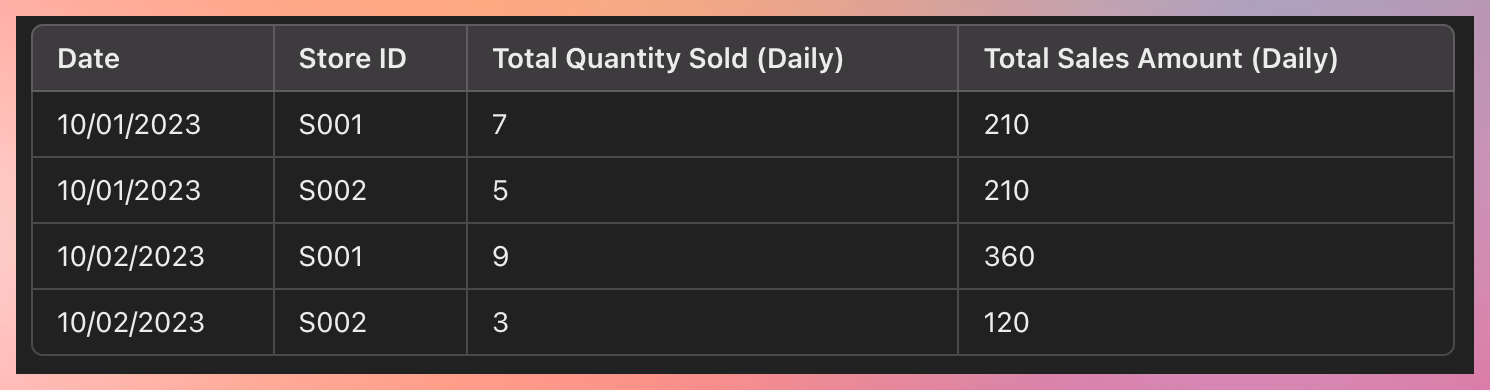
Use Case:
- Analyze business performance at a fixed interval.
- Status of all flights.
- Inventory stock. How much stock is left at the end of the day?
Transaction Fact Table is the source, and this stores a snapshot of info.
GRAIN for this table will be hourly / 2 hrs / daily based on need.
Accumulating Snapshot Fact Table
An Accumulating Snapshot Fact Table is used to track processes or workflows that have a definite beginning and end but take place over time. It allows you to capture the state of a process at different stages and update facts as the process progresses.
A classic example of an accumulating snapshot is in the order processing workflow, where we track the progress of an order from placement through to fulfillment and shipping. The fact table accumulates data as each order moves through various stages.
Amazon Order.. what happened at several time intervals.
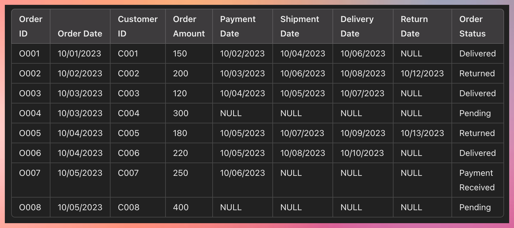
As the process moves from one step to another, these get updated.
Accumulating snapshot always has different date fields denoting multiple stages of the process.
Use Cases
Track Returns: You can easily track which orders have been returned by checking the Return Date and filtering by Order Status = "Returned."
Monitor the Order Workflow: You can monitor the progress of orders through the entire workflow by checking how long it takes from Order Date to Payment Date, Shipment Date, Delivery Date, and Return Date (if applicable).
Calculate Performance Metrics: Calculate metrics like average delivery time, return rates, or the percentage of orders that are still pending or awaiting shipment.
Example Queries
Find all returned orders: Query for orders where Return Date is not NULL.
Calculate time from order to delivery: Subtract Order Date from Delivery Date to calculate how long deliveries take.
Track pending orders: Filter where Order Status is "Pending" or Shipment Date is NULL.
Another example: Hospital entry
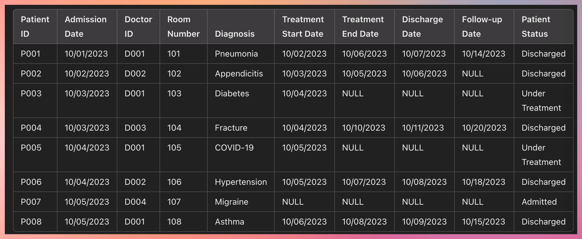
How the Accumulating Snapshot Works:
Row Creation: A new row is created when the patient is admitted, with basic information like Admission Date, Doctor ID, and Diagnosis.
Row Updates: As the patient's treatment progresses, additional fields like Treatment Start Date, Treatment End Date, Discharge Date, and Follow-up Date are updated.
Transaction vs Periodic vs Accumulating
Difference between 3 Fact Tables
| Transaction | Periodic | Accumulating |
|---|---|---|
| Stores lowest grain of data. | Stores current state of data at a regular interval of time. | Stores intermediate steps that has happened over a period of time. |
| one row per Transaction | one row per time period | one row per entire lifetime of the event |
| Date dimension is lowest table | Date/time is regular interval of snapshot frequency | multiple data dimensions for intermediate steps |
| Easy to aggregate | minimal aggregation | not easy to aggregate |
| largest database size | Medium Database size | Smallest Database Size |
| Only Insert | Only Insert | Insert and Update |
| Most business requirement | business performance is reviewed at regular interval | the Business process has multiple stages |
Additive, Semi-Additive, Non-Additive
In data warehousing, a fact table contains measurements or facts, which can be categorized into three types: additive, semi-additive, and non-additive.
Additive Facts
These can be summed across all dimensions of the fact table. Additive facts are the most straightforward to aggregate and are commonly used in reporting.
Examples:
- Sales revenue: Can be summed by time, product, region, etc.
- Quantity sold: Summable across product, time, store dimensions.
- Profit: Aggregates well across dimensions.
- Number of website visits: Can be summed up by day, user, or region.
- Number of clicks on a banner ad: Can be aggregated across time, campaigns, etc.
Semi-Additive Facts
These can be summed across some dimensions but not others. For example, summing across time might not make sense for certain facts like balances or inventory, which are snapshot-based.
Examples:
- Bank balance: Can be summed across accounts but not over time (as balances are snapshots at specific points in time).
- Stock price: Cannot be summed across time but might be relevant for a single stock across locations or markets.
- Inventory levels: Summable across product or location but not over time. Number of employees: Summable by department, but not over time as it's a snapshot metric.
- Number of students enrolled in a course: Summable by course but not over time.
Non-Additive Facts
These cannot be summed across any dimension. These are usually metrics like ratios, percentages, or averages that do not make sense to sum.
Examples:
- Profit margin: It's a ratio and cannot be added up across regions or time.
- Gross margin percentage: Like profit margin, it’s a percentage and non-additive.
- Average temperature: Averages do not sum well; they need to be recalculated for larger groups.
- Average customer satisfaction rating: Cannot sum up ratings; they need to be averaged again for larger sets.
- Percentage of market share: Similar to margins, percentages cannot be summed.
It is essential to identify the type of fact as it determines how the fact table will be aggregated and also impacts the design of the data warehouse.
Example
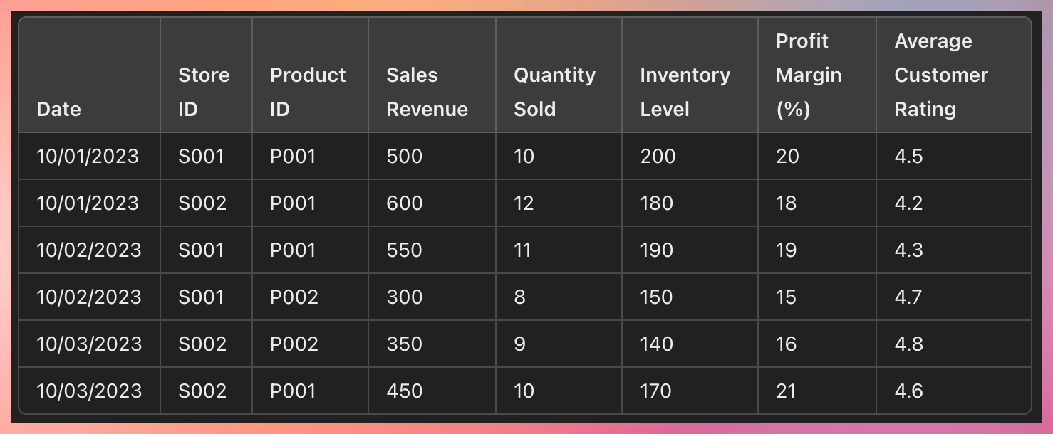
Additive Facts:
Sales Revenue: Can be summed across all dimensions (e.g., total sales revenue by day, store, product, etc.). Quantity Sold: Additive across all dimensions (e.g., sum of quantities sold by product, store, or day).
Total Sales Revenue for P001 across all stores on 10/01/2023 = 500 (S001) + 600 (S002) = 1100.
Total Quantity Sold for P001 on 10/01/2023 = 10 (S001) + 12 (S002) = 22.
Semi-Additive Facts:
Inventory Level: This represents a snapshot of inventory at a given time. You can sum inventory across stores but not across time (e.g., you can sum inventory for a product across different stores at a single point in time, but not over multiple days).
Inventory Level for P001 on 10/01/2023 across all stores = 200 (S001) + 180 (S002) = 380.
Inventory Level across time would not be summed (e.g., you cannot add inventory levels on 10/01 and 10/02).
Non-Additive Facts:
Profit Margin (%): Cannot be summed across any dimension, as it is a percentage. For example, adding profit margins across stores or products would not yield a meaningful result. Instead, you'd need to compute a weighted average.
Average Customer Rating: Similar to profit margin, it cannot be summed across stores or time. It would need to be recalculated as an average if you wanted to aggregate it.
Average Profit Margin for P001 on 10/01/2023 would need to be recalculated based on weighted averages of sales revenues or units sold.
Average Customer Rating would need to be recalculated based on customer reviews or feedback.
Periodic Snapshot vs Additive
Periodic snapshot fact and additive fact are different concepts, although they may appear similar at first glance.
A periodic snapshot fact table is designed to capture a point-in-time snapshot of some measure at regular intervals, typically periodically, such as daily, weekly, monthly, or quarterly.
An additive fact represents a measure that can be aggregated across all dimensions in a fact table. For example, sales revenue is an additive fact because it can be summed up across all dimensions such as time, product, region, etc.
| Additive Fact | Periodic Snapshot Fact | |
|---|---|---|
| Definition | Represents a measure that can be aggregated across all dimensions in a fact table | Captures a point-in-time snapshot of some measure at regular intervals |
| Granularity | Can be at any level of granularity | Usually at a higher level of granularity such as daily, weekly, monthly, or quarterly |
| Aggregation | Can be summed up across all dimensions in the fact table | Captures the total value of the measure at a specific point in time |
| Example | Sales revenue, profit, number of clicks on a banner ad | Monthly sales revenue, quarterly website visits, daily customer support tickets |
Conformed Fact
The fact is used in more than one fact table. (Attribute)
The conformed Fact table is a fact table that can be used across multiple Data Marts.
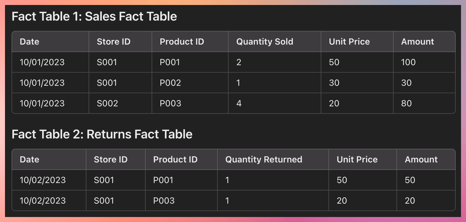
Suppose a company has separate fact tables for Online Sales and In-store Sales. Both these fact tables might have a "Total Sales" metric.
To ensure that this metric is a conformed fact, the company would need to make sure that "Total Sales" has the same meaning (i.e., the total revenue from sales), the same scale (e.g., in US dollars), and is calculated in the same way (e.g., quantity sold times unit price) in both fact tables.
Miscellaneous
- CSV to Dimension Models Example
- Data Architecture Diagram
- Data Pipeline Models
- New DW Concepts
- Dataset Examples
- Thoughts on some data
CSV to Dimension Models Example
Sample Data
https://github.com/gchandra10/filestorage/blob/main/sales_100.csv
Design using https://mermaid.live/
---
title: Sales 100 example
---

erDiagram
  dim_region {
    region_id int
    region_name string
  }

  dim_country {
    country_id int
    region_id int
    country_name string
  }

  dim_item_type {
    item_type_id int
    item_type_name string
  }

  dim_sales_channel {
    sales_channel_id int
    sales_channel_type string
  }

  dim_order_priority{
    order_priority_id int
    order_priority string
  }

  dim_date{
    date_id int
    shortdate date
    day_of_week string
    is_weekend boolean
    day int
    month int
    week_of_month int
    week_of_year int
    quarter string
    year int
    leap_year boolean
  }

  fact_order_transaction {
    id int
    order_id int
    country_id int
    item_type_id int
    sales_channel_id int
    order_priority_id int

    order_date_id int
    ship_date_id int

    units_sold int
    unit_price float
    unit_cost float
    total_revenue float
    total_cost float
    total_profit float
  }

  dim_month {
    month_id int pk
    month string
    year int
    quarter string
    is_end_of_year boolean
  }

  fact_quarterly_sales {
    id int
    month_id int
    total_units_sold int
    total_revenue float
    total_cost float
    total_profit float
  }

  fact_region_sales{
    id int
    region_id int
    sales_channel_id int
    total_units_sold int
    total_revenue float
    total_cost float
    total_profit float
  }

dim_region ||--o{ dim_country : "region_id"
dim_country ||--o{ fact_order_transaction : "country_id"
dim_item_type ||--o{ fact_order_transaction : "item_type_id"
dim_sales_channel ||--o{ fact_order_transaction : "sales_channel_id"
dim_order_priority  ||--o{ fact_order_transaction : "order_priority_id"
dim_date ||--o{ fact_order_transaction : "order_date"
dim_date ||--o{ fact_order_transaction : "ship_date"

dim_month ||--o{ fact_quarterly_sales : "month_id"

dim_region ||--o{ fact_region_sales : "region_id"
dim_sales_channel ||--o{ fact_region_sales : "sales_channel_id"
Design
---
title: Sales 100 example
---

erDiagram
  dim_region {
    region_id int
    region_name string
  }

  dim_country {
    country_id int
    region_id int
    country_name string
  }

  dim_item_type {
    item_type_id int
    item_type_name string
  }

  dim_sales_channel {
    sales_channel_id int
    sales_channel_type string
  }

  dim_order_priority{
    order_priority_id int
    order_priority string
  }

  dim_date{
    date_id int
    shortdate date
    day_of_week string
    is_weekend boolean
    day int
    month int
    week_of_month int
    week_of_year int
    quarter string
    year int
    leap_year boolean
  }

  fact_order_transaction {
    id int
    order_id int
    country_id int
    item_type_id int
    sales_channel_id int
    order_priority_id int

    order_date_id int
    ship_date_id int

    units_sold int
    unit_price float
    unit_cost float
    total_revenue float
    total_cost float
    total_profit float
  }

  dim_month {
    month_id int pk
    month string
    year int
    quarter string
    is_end_of_year boolean
  }

  fact_quarterly_sales {
    id int
    month_id int
    total_units_sold int
    total_revenue float
    total_cost float
    total_profit float
  }

  fact_region_sales{
    id int
    region_id int
    sales_channel_id int
    total_units_sold int
    total_revenue float
    total_cost float
    total_profit float
  }

dim_region ||--o{ dim_country : "region_id"
dim_country ||--o{ fact_order_transaction : "country_id"
dim_item_type ||--o{ fact_order_transaction : "item_type_id"
dim_sales_channel ||--o{ fact_order_transaction : "sales_channel_id"
dim_order_priority  ||--o{ fact_order_transaction : "order_priority_id"
dim_date ||--o{ fact_order_transaction : "order_date"
dim_date ||--o{ fact_order_transaction : "ship_date"

dim_month ||--o{ fact_quarterly_sales : "month_id"

dim_region ||--o{ fact_region_sales : "region_id"
dim_sales_channel ||--o{ fact_region_sales : "sales_channel_id"
Sample Data Architecture Diagram
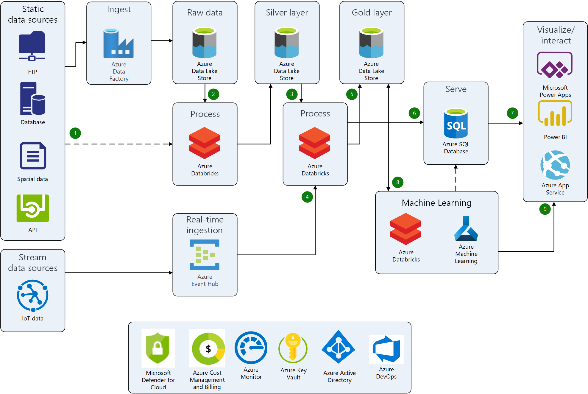
https://learn.microsoft.com/en-us/azure/architecture/example-scenario/analytics/sports-analytics-architecture-azure
How do you draw architectural diagrams?
Data Pipeline Models
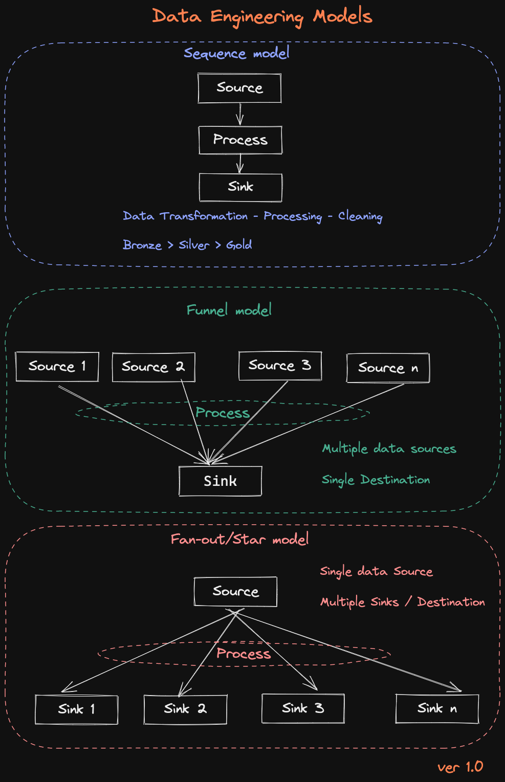
Sequence Model
The Sequence Model represents a linear flow where data moves from a Source to a Process stage and finally to a Sink. This model is ideal for straightforward data transformations and processing tasks, where data is ingested, cleaned, and transformed sequentially before being stored in the final destination. This approach aligns with the traditional Bronze → Silver → Gold layer strategy in data engineering.
Funnel Model
After processing, the Funnel Model aggregates data from multiple sources into a single Sink. This model is useful when combining data from various origins, such as multiple databases or external APIs, into a unified repository. The central processing stage consolidates and harmonizes data from these different sources before loading it into the destination, ensuring that data from diverse inputs is integrated into one output.
Fan-out/Star Model
The Fan-out/Star Model starts with a single Source, processes the data, and then distributes the results to multiple Sinks. This model is effective when the processed data needs to be utilized in various downstream applications or systems. It allows the same source data to be transformed and delivered to different destinations, each serving a unique purpose or system requirement.
Each model serves distinct data engineering needs, from simple data pipelines to complex ETL processes involving multiple sources or destinations.
New DW Concepts
- Cloud Data Warehousing: With the increasing popularity of cloud computing, cloud data warehousing has become a popular concept. It involves storing data in a cloud-based rather than an on-premise data warehouse. This allows for greater scalability, flexibility, and cost savings.
Examples: Databricks, Snowflake, Azure Synapse, and so on.
-
Data Virtualization: Data virtualization is a technique that allows data to be accessed and integrated from multiple sources without the need for physical data movement or replication. This can help reduce data redundancy and improve data consistency.
-
Self-Service BI: Self-service BI allows business users to access and analyze data without relying on IT or data analysts. This concept has become popular with user-friendly data visualization tools enabling users to create reports and dashboards.
-
Big Data Analytics: Big data analytics involves using advanced analytics techniques to analyze large and complex datasets. This requires specialized tools and technologies, such as Hadoop and Spark, to process and analyze large volumes of data.
-
Data Governance: Data governance involves establishing policies, standards, and procedures for managing data assets. This helps ensure data accuracy, consistency, and security and that data is used to align with organizational goals and objectives.
-
Delta Sharing: With Delta Sharing, organizations can share their data with partners, customers, and other stakeholders without having to move or copy the data. This can help reduce data duplication and improve data governance while allowing for more collaborative and agile data sharing.
Overall, these new data warehousing concepts are focused on improving the speed, flexibility, and accessibility of data and ensuring that data is used in a way that supports organizational objectives.
-
DataOps: DataOps is a methodology that emphasizes collaboration, automation, and monitoring to improve the speed and quality of data analytics. It combines DevOps and agile methods to create a more efficient and streamlined data pipeline.
-
Data Mesh: Data Mesh is an architectural approach emphasizing decentralization and domain-driven data architecture design. It involves breaking down data silos and creating a more flexible and scalable data architecture that aligns with business needs.
-
Augmented Analytics: Augmented analytics is a technique that uses machine learning and artificial intelligence to automate data preparation, insight generation, and insight sharing. It aims to improve the speed and accuracy of data analytics while reducing the reliance on data scientists and analysts.
-
Real-time Data Warehousing: Real-time data warehousing involves using streaming data technologies like Apache Kafka to capture and process data in real-time. This enables organizations to analyze and act on data in real-time rather than waiting for batch processing cycles.
-
Data Privacy and Ethics: Data privacy and ethics are becoming increasingly important in data warehousing and analytics. Organizations focus on ensuring that data is collected, stored, and used ethically and responsibly and that data privacy regulations, such as GDPR and CCPA, are followed.
These are just a few new data warehousing concepts emerging in response to the changing data landscape. As data volumes continue to grow and technologies continue to evolve, we can expect to see continued innovation in data warehousing and analytics.
Dataset Examples
Retail Sales Transactions: This dataset includes individual retail store or chain sales transactions. It typically contains transaction ID, customer ID, product ID, quantity, price, and timestamp.
| Transaction ID | Customer ID | Product | Quantity | Price | Timestamp |
|---|---|---|---|---|---|
| T001 | C001 | Apple iPhone X | 5 | $10.99 | 2023-05-10 10:30:15 |
| T002 | C002 | Samsung Galaxy S9 | 3 | $24.99 | 2023-05-10 14:45:21 |
| T003 | C003 | HP Printer | 2 | $5.99 | 2023-05-11 09:12:33 |
Financial Transactions: This dataset consists of financial transactions from banks or credit card companies. It includes transaction ID, account number, transaction type, amount, merchant information, and timestamp.
| Transaction ID | Account Number | Transaction Type | Amount | Merchant | Timestamp |
|---|---|---|---|---|---|
| T001 | A123456 | Deposit | $100.00 | XYZ Bank | 2023-05-10 08:15:30 |
| T002 | B987654 | Withdrawal | -$50.00 | ABC Store | 2023-05-10 15:20:45 |
| T003 | C246810 | Transfer | $250.00 | Online Shopping | 2023-05-11 11:05:12 |
Online Marketplace Transactions: This dataset contains transactions from an online marketplace like Amazon, eBay, or Alibaba. It includes transaction ID, buyer/seller ID, product ID, quantity, price, shipping details, and timestamps.
| Transaction ID | Buyer | Seller | Product | Quantity | Price | Shipping Details | Timestamp |
|---|---|---|---|---|---|---|---|
| T001 | John Doe | SellerA | Book | 1 | $19.99 | Address1, City1, State1 | 2023-05-10 13:45:27 |
| T002 | Jane Smith | SellerB | Smartphone | 2 | $49.99 | Address2, City2, State2 | 2023-05-10 16:20:10 |
| T003 | Mark Johnson | SellerC | Headphones | 3 | $9.99 | Address3, City3, State3 | 2023-05-11 10:05:55 |
E-commerce Order Transactions: This dataset focuses on transactions from an e-commerce website. It includes data such as order ID, customer ID, product ID, quantity, price, shipping information, payment details, and timestamps.
| Order ID | Customer | Product | Quantity | Price | Shipping Information | Payment Details | Timestamp |
|---|---|---|---|---|---|---|---|
| O001 | John Doe | Apple iPhone X | 2 | $29.99 | Address1, City1, State1 | Credit Card | 2023-05-10 11:30:45 |
| O002 | Jane Smith | Samsung Galaxy S9 | 1 | $14.99 | Address2, City2, State2 | PayPal | 2023-05-10 17:15:20 |
| O003 | Mark Johnson | HP Printer | 4 | $39.99 | Address3, City3, State3 | Credit Card | 2023-05-11 08:45:10 |
Travel Booking Transactions: This dataset comprises transactions from a travel booking website or agency. It includes booking ID, traveler details, flight/hotel ID, dates, prices, payment information, and timestamps.
| Booking ID | Traveler | Flight | Hotel | Dates | Price | Payment Information | Timestamp |
|---|---|---|---|---|---|---|---|
| B001 | John Doe | Flight 123 | Hotel ABC | 2023-06-15 - 2023-06-20 | $500.00 | Credit Card | 2023-05-10 09:30:15 |
| B002 | Jane Smith | Flight 456 | Hotel XYZ | 2023-07-01 - 2023-07-10 | $750.00 | PayPal | 2023-05-11 14:20:30 |
| B003 | Mark Johnson | Flight 789 | Hotel PQR | 2023-08-10 - 2023-08-15 | $600.00 | Credit Card | 2023-05-12 11:45:55 |
Stock Market Transactions: This dataset involves transactions from stock exchanges. It includes details like trade ID, stock symbol, buy/sell order, quantity, price, trader information, and timestamps.
| Transaction ID | Stock Symbol | Buy/Sell | Quantity | Price | Trader | Timestamp |
|---|---|---|---|---|---|---|
| T001 | AAPL | Buy | 100 | $150.50 | John Doe | 2023-05-10 09:30:15 |
| T002 | GOOGL | Sell | 50 | $2500.00 | Jane Smith | 2023-05-10 11:15:45 |
| T003 | MSFT | Buy | 75 | $180.75 | Mark Johnson | 2023-05-10 14:40:20 |
Datasets
https://cseweb.ucsd.edu/~jmcauley/datasets.html
Popular API Sources
- https://developer.spotify.com/documentation/web-api
- https://developer.marvel.com/
- https://developers.google.com/youtube/
- https://www.openfigi.com/api
Thoughts on data
Don't remove NULL columns or Bad data from the Source. Learn to handle that in processing.
Sample 1
| Serial_Number | List_Year | Code |
|---|---|---|
| 20093 | 2020 | 10 - A Will |
| 200192 | 2020 | 14 - Foreclosure |
| 190871 | 2019 | 18 - In Lieu Of Foreclosure |
Create a separate Dimension table for Code and split the Code No and Code Name
| dim_code |
|---|
| id |
| code_no |
| code_name |
| fact |
|---|
| Serial_Number |
| List_Year |
| dim_id |
Sample 2
| TripID | Source Lat | Source Long | Des Lat | Des Long |
|---|---|---|---|---|
| 1 | -73.9903717 | 40.73469543 | -73.98184204 | 40.73240662 |
| 2 | -73.98078156 | 40.7299118 | -73.94447327 | 40.71667862 |
| 3 | -73.98455048 | 40.67956543 | -73.95027161 | 40.78892517 |
Separate Dimension for Lat and Long
| dim_location |
|---|
| location_id |
| lat |
| long |
| location_name (If exists) |
Updated Fact table
| fact |
|---|
| trip_id |
| source_location_id |
| destination_location_id |
Another Variation
| Location |
|---|
| POINT (-72.98492 41.64753) |
| POINT (-72.96445 41.25722) |
Notes:
DRY Principle: You're not repeating the lat-long info, adhering to the "Don't Repeat Yourself" principle.
Ease of Update: If you need to update a location's details, you do it in one place.
Flexibility: Easier to add more attributes to locations in the future.
5 decimal places: Accurate to ~1.1 meters, usually good enough for most applications including vehicle navigation.
4 decimal places: Accurate to ~11 meters, may be suitable for some applications but not ideal for vehicle-level precision.
3 decimal places: Accurate to ~111 meters, generally too coarse for vehicle navigation but might be okay for city-level analytics.
Sample 3
| Fiscal Year | Disbursement Date | Vendor Invoice Date | Vendor Invoice Week | Check Clearance Date |
|---|---|---|---|---|
| 2023 | 06-Oct-23 | 08-Aug-23 | 08-06-2023 | |
| 2023 | 06-Oct-23 | 16-Aug-23 | 08/13/2023 | |
| 2023 | 06-Oct-23 | 22-Sep-23 | 09/17/2023 | 10-08-2023 |
Date Dimension
| DateKey | FullDate | Year | Month | Day | Weekday | WeekOfYear | Quarter | IsWeekend | IsHoliday |
|---|---|---|---|---|---|---|---|---|---|
| 20230808 | 2023-08-08 | 2023 | 8 | 8 | 2 | 32 | 3 | FALSE | FALSE |
| 20230816 | 2023-08-16 | 2023 | 8 | 16 | 3 | 33 | 3 | FALSE | FALSE |
| 20230922 | 2023-09-22 | 2023 | 9 | 22 | 5 | 38 | 3 | FALSE | FALSE |
| 20231006 | 2023-10-06 | 2023 | 10 | 6 | 5 | 40 | 4 | FALSE | FALSE |
| 20231008 | 2023-10-08 | 2023 | 10 | 8 | 7 | 40 | 4 | TRUE | FALSE |
| ... | ... | ... | ... | ... | ... | ... | ... | ... | ... |
Fact Table
| Fiscal Year | Disbursement Date Key | Vendor Invoice Date Key | Vendor Invoice Week Date Key | Check Clearance Date Key |
|---|---|---|---|---|
| 2023 | 20231006 | 20230808 | 20230806 | |
| 2023 | 20231006 | 20230816 | 20230813 | |
| 2023 | 20231006 | 20230922 | 20230917 | 20231008 |
Sample 4
Another DateTime
| date_attending | ip_location |
|---|---|
| 2017-12-23 12:00:00 | Reseda, CA, United States |
| 2017-12-23 12:00:00 | Los Angeles, CA, United States |
| 2018-01-05 14:00:00 | Mission Viejo, CA, United States |
Date Time Dimension
| DateKey | FullDate | Year | Month | Day | Weekday | WeekOfYear | Quarter | IsWeekend | IsHoliday |
|---|---|---|---|---|---|---|---|---|---|
| 20171223 | 2017-12-23 | 2017 | 12 | 23 | 6 | 51 | 4 | TRUE | FALSE |
| 20180105 | 2018-01-05 | 2018 | 1 | 5 | 5 | 1 | 1 | FALSE | FALSE |
| ... | ... | ... | ... | ... | ... | ... | ... | ... | ... |
Fact Table
| FactID | DateKey | ip_location |
|---|---|---|
| 1 | 20171223 | Reseda, CA, United States |
| 2 | 20171223 | Los Angeles, CA, United States |
| 3 | 20180105 | Mission Viejo, CA, United States |
Sample 5
| Job Title | Experience | Qualifications | Salary Range | Age_Group |
|---|---|---|---|---|
| Digital Marketing Specialist | 5 to 15 Years | M.Tech | $59K-$99K | Youth (<25) |
| Web Developer | 2 to 12 Years | BCA | $56K-$116K | Adults (35-64) |
| Operations Manager | 0 to 12 Years | PhD | $61K-$104K | Young Adults (25-34) |
| Network Engineer | 4 to 11 Years | PhD | $65K-$91K | Young Adults (25-34) |
| Event Manager | 1 to 12 Years | MBA | $64K-$87K | Adults (35-64) |
Experience Dimension
| ExperienceID | ExperienceRange | MinExperience | MaxExperience |
|---|---|---|---|
| 1 | 5 to 15 Years | 5 | 15 |
| 2 | 2 to 12 Years | 2 | 12 |
| 3 | 0 to 12 Years | 0 | 12 |
| 4 | 4 to 11 Years | 4 | 11 |
| 5 | 1 to 12 Years | 1 | 12 |
Job Dimension Table
| JobID | Job Title | Qualifications |
|---|---|---|
| 1 | Digital Marketing Specialist | M.Tech |
| 2 | Web Developer | BCA |
| 3 | Operations Manager | PhD |
| 4 | Network Engineer | PhD |
| 5 | Event Manager | MBA |
Age Group Dimension Table
| AgeGroupID | Age_Group |
|---|---|
| 1 | Youth (<25) |
| 2 | Adults (35-64) |
| 3 | Young Adults (25-34) |
Fact Table
| JobID | ExperienceID | Salary Range | AgeGroupID |
|---|---|---|---|
| 1 | 1 | $59K-$99K | 1 |
| 2 | 2 | $56K-$116K | 2 |
| 3 | 3 | $61K-$104K | 3 |
| 4 | 4 | $65K-$91K | 3 |
| 5 | 5 | $64K-$87K | 2 |
Sample 6
| ITEM CODE | ITEM DESCRIPTION |
|---|---|
| 100293 | SANTORINI GAVALA WHITE - 750ML |
| 100641 | CORTENOVA VENETO P/GRIG - 750ML |
| 100749 | SANTA MARGHERITA P/GRIG ALTO - 375ML |
The Fact will turn out to be like this
| ItemID | ItemCode | Item Description | Quantity |
|---|---|---|---|
| 1 | 100293 | SANTORINI GAVALA WHITE | 750ML |
| 2 | 100641 | CORTENOVA VENETO P/GRIG | 750ML |
| 3 | 100749 | SANTA MARGHERITA P/GRIG ALTO | 375ML |
Note: If the same Item Descrition repeats for various quantities, then create a separate table for Quantity.
Quantity Dimension
| QuantityID | Quantity |
|---|---|
| 1 | 750ML |
| 2 | 375ML |
| 3 | 500ML |
| ... | ... |
Item Dimension
| ItemID | Item Name | QuantityID |
|---|---|---|
| 1 | SANTORINI GAVALA WHITE | 1 |
| 2 | CORTENOVA VENETO P/GRIG | 1 |
| 3 | SANTA MARGHERITA P/GRIG ALTO | 2 |
| ... | ... | ... |
Fact Table
| FactID | ItemID | QuantityID |
|---|---|---|
| 1 | 1 | 1 |
Sample 7
| production_countries | spoken_languages |
|---|---|
| United Kingdom, United States of America | English, French, Japanese, Swahili |
| United Kingdom, United States of America | English |
| United Kingdom, United States of America | English, Mandarin |
Country Dimension
| CountryID | CountryName |
|---|---|
| 1 | United Kingdom |
| 2 | United States of America |
Language Dimension
| LanguageID | LanguageName |
|---|---|
| 1 | English |
| 2 | French |
| 3 | Japanese |
| 4 | Swahili |
| 5 | Mandarin |
Approach 1 : Creating Many to Many
| FactID | CountryID | LanguageID |
|---|---|---|
| 1 | 1 | 1 |
| 1 | 2 | 1 |
| 1 | 1 | 2 |
| 1 | 2 | 2 |
Pros
Normalization: Easier to update and maintain data.
Cons
Storage: May require more storage for the additional tables and keys.
Approach 2 : Fact Table with Array Datatypes
| FactID | ProductionCountryIDs | SpokenLanguageIDs |
|---|---|---|
| 1 | [1, 2] | [1, 2, 3, 4] |
| 2 | [1, 2] | [1] |
| 3 | [1, 2] | [1, 5] |
With newer Systems like Spark SQL which supports Arrays
- Simplicity: Easier to understand and less complex to set up.
- Performance: Could be faster for certain types of queries, especially those that don't require unpacking the array.